
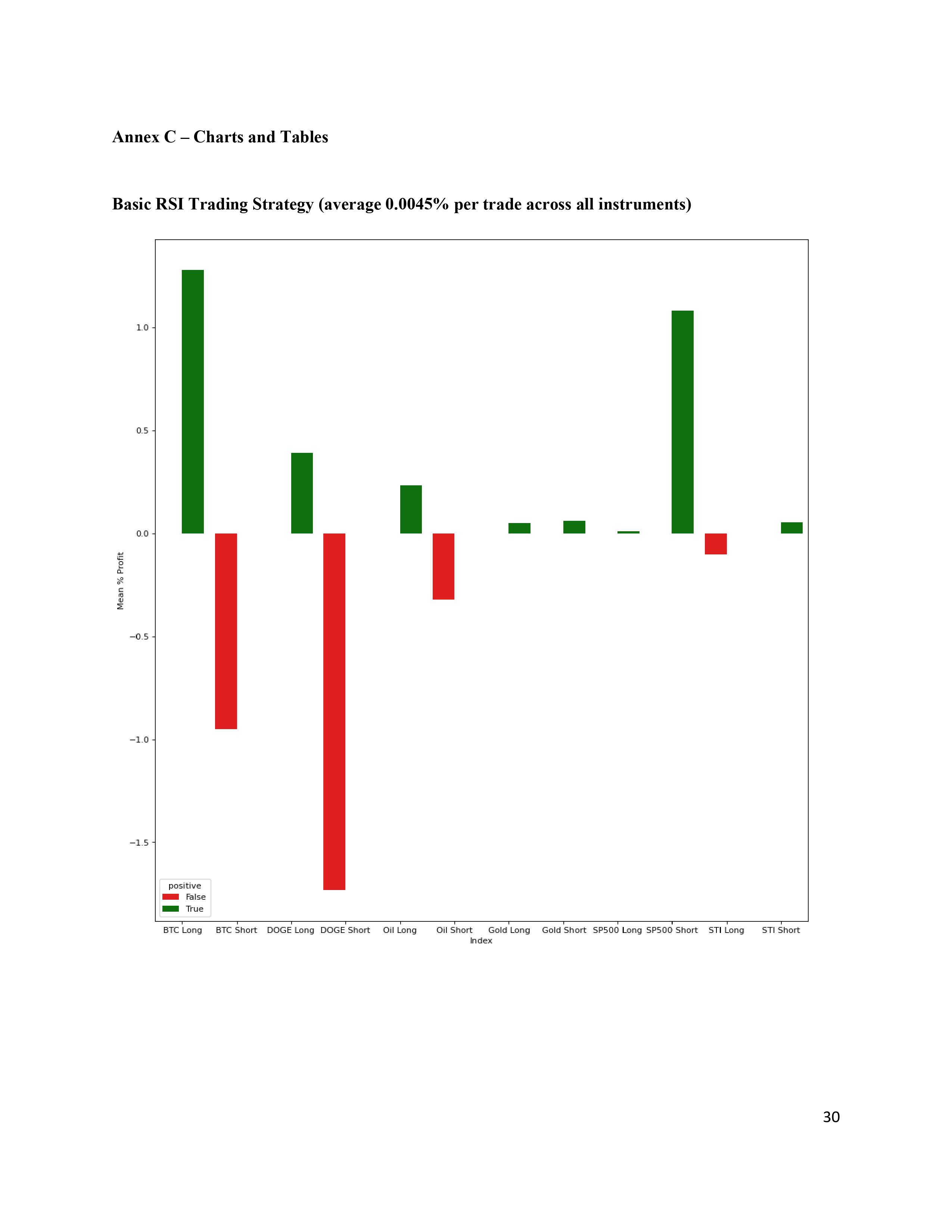
Statistics | Autoregressive Distributed Lag Model | Trading Strategies | Backtesting
This project was completed as part of the Statistics Module at SMU based on the Introduction to Econometrics, Global 4th Edition (2020) textbook. The course covered different ways of modelling and determining the fit of models based purely on statistics and gave me a deep understanding of the roots and concepts behind which current machine learning models were built upon. In terms of value, it develops a workflow for quickly determining the profitability of simple trading strategies through both the engineering of the data and backtesting of results.
From the perspective of someone who has worked with multiple machine learning models before this module, I found that the statistical method of developing models was often more tedious in both setting up the data and applying the correct model for the specific context. However the major advantage came in the form of interpretability of the model's fit (especially for simpler models like the Ordinary Least Squares Regression Models). The array of model parameters that are generated after the fit quantifies how well a model fits the data from different angles (error, mean, variance, lags) which are invaluable for interpretation and understanding the limitations of the model. This is (currently) often lacking for machine learning models.
The report explaining the project is as seen below. As my group was busy working on other projects, most of the programming and writing was completed by me.


The contents of the notebook appended below dive straight into the first of 5 stages:
import pandas as pd

        sti_df = pd.read_csv('STI (Singapore).csv')
sti_df
| Date | Open | High | Low | Close | |
|---|---|---|---|---|---|
| 0 | 10/08/21 | 3110.82 | 3112.81 | 3112.81 | 3112.81 |
| 1 | 10/07/21 | 3099.99 | 3118.52 | 3098.81 | 3101.15 |
| 2 | 10/06/21 | 3082.58 | 3091.35 | 3066.38 | 3083.88 |
| 3 | 10/05/21 | 3071.93 | 3071.93 | 3047.38 | 3068.12 |
| 4 | 10/04/21 | 3079.99 | 3102.47 | 3079.62 | 3089.65 |
| ... | ... | ... | ... | ... | ... |
| 942 | 01/08/18 | 3498.62 | 3514.76 | 3494.54 | 3512.18 |
| 943 | 01/05/18 | 3502.34 | 3503.68 | 3480.22 | 3489.45 |
| 944 | 01/04/18 | 3476.43 | 3501.16 | 3465.95 | 3501.16 |
| 945 | 01/03/18 | 3434.70 | 3468.19 | 3432.87 | 3464.28 |
| 946 | 01/02/18 | 3406.48 | 3433.82 | 3403.87 | 3430.30 |
947 rows × 5 columns
sti_df.columns
Index(['Date', 'Open', 'High', 'Low', 'Close', 'Volume'], dtype='object')
import talib
        import numpy as np

        sti_rsi = talib.RSI(sti_df[' Close'], timeperiod=14)

        d = {'Date': sti_df['Date'], ' RSI': sti_rsi}
        sti_rsi_df = pd.DataFrame(data=d)
        sti_rsi_df['RSI Condition'] = sti_rsi_df[' RSI'].copy()

        sti_rsi_df[' Close'] = sti_df[' Close']
        sti_rsi_df.loc[sti_rsi_df['RSI Condition'] <= 30, 'RSI Condition'] = 1
        sti_rsi_df.loc[(sti_rsi_df['RSI Condition'] > 30) & (sti_rsi_df['RSI Condition'] < 70), 'RSI Condition'] = 0
        sti_rsi_df.loc[sti_rsi_df['RSI Condition'] >= 70, 'RSI Condition'] = -1
        sti_rsi_df[' RSI'] = sti_rsi_df[' RSI']*30
sti_rsi_df.describe()
| RSI | RSI Condition | Close | |
|---|---|---|---|
| count | 933.000000 | 933.000000 | 947.00000 |
| mean | 1497.511185 | -0.011790 | 3084.51773 |
| std | 370.906023 | 0.325705 | 293.85772 |
| min | 378.636955 | -1.000000 | 2233.48000 |
| 25% | 1232.309343 | 0.000000 | 2973.59500 |
| 50% | 1507.572202 | 0.000000 | 3156.28000 |
| 75% | 1761.470849 | 0.000000 | 3247.51500 |
| max | 2435.438332 | 1.000000 | 3615.28000 |
import matplotlib.pyplot as plt
        import numpy as np
        import seaborn as sns

        fig, ax = plt.subplots(figsize=(14, 15), dpi=80)

        color_dict = dict({0:'black',
                            1:'green',
                          -1: 'red'})

        markers = dict({0:'o',
                        1:'^',
                        -1: 'v'})

        size_dict = dict({0:3,
                          1:100,
                          -1:100})

        p0 = sns.lineplot(data=sti_df, x="Date", y="Close", ax=ax)
        p1 = sns.lineplot(data=sti_rsi_df, x="Date", y=" RSI", label='RSI Condition', ax=ax)
        p3 = sns.scatterplot(data=sti_rsi_df, x= "Date", y=' Close', hue ='RSI Condition', palette=color_dict, style='RSI Condition', markers=markers, size='RSI Condition', sizes=size_dict, ax=ax)
        p5 = sns.lineplot(data=sti_ema_df, x="Date", y=" EMA200", ax=ax)

sti_macd, sti_macdsignal, sti_macdhist = talib.MACD(sti_df[' Close'], fastperiod=12, slowperiod=26, signalperiod=9)

        d = {'Date': sti_df['Date'], ' MACD': sti_macd, ' MACD_SIG': sti_macdsignal}
        sti_macd_df = pd.DataFrame(data=d)
        sti_macd_df['MACD Condition'] = 0

        for df_entry in range(len(sti_macd_df)-1):
            #MACD crossing MACD_SIGNAL from above
            if sti_macd_df[' MACD'][df_entry] > sti_macd_df[' MACD_SIG'][df_entry] and sti_macd_df[' MACD'][df_entry+1] < sti_macd_df[' MACD_SIG'][df_entry+1]:
                sti_macd_df['MACD Condition'][df_entry] = -1
                #print(sti_macd_df[' MACD'][df_entry],sti_macd_df[' MACD_SIG'][df_entry],sti_macd_df[' MACD'][df_entry+1],sti_macd_df[' MACD_SIG'][df_entry+1])
            #MACD crossing MACD_SIGNAL from below
            if sti_macd_df[' MACD'][df_entry] < sti_macd_df[' MACD_SIG'][df_entry] and sti_macd_df[' MACD'][df_entry+1] > sti_macd_df[' MACD_SIG'][df_entry+1]:
                sti_macd_df['MACD Condition'][df_entry] = 1
                #print(sti_macd_df[' MACD'][df_entry],sti_macd_df[' MACD_SIG'][df_entry],sti_macd_df[' MACD'][df_entry+1],sti_macd_df[' MACD_SIG'][df_entry+1])

        sti_macd_orders_df = sti_macd_df.loc[sti_macd_df['MACD Condition'] != 0]
        sti_macd_orders_df[' Close'] = sti_df[' Close']
        sti_macd_orders_df
| Date | MACD | MACD_SIG | MACD Condition | Close | |
|---|---|---|---|---|---|
| 48 | 08/02/21 | 22.884501 | 22.061499 | -1 | 3161.22 |
| 78 | 06/18/21 | -4.643763 | -4.378131 | 1 | 3144.16 |
| 94 | 05/27/21 | 9.306626 | 8.015733 | -1 | 3164.82 |
| 104 | 05/11/21 | -9.995296 | -6.626359 | 1 | 3144.27 |
| 117 | 04/22/21 | 16.693823 | 14.232237 | -1 | 3187.78 |
| 129 | 04/06/21 | 7.638559 | 8.541848 | 1 | 3207.63 |
| 130 | 04/05/21 | 8.593651 | 8.552209 | -1 | 3209.74 |
| 163 | 02/16/21 | -58.695592 | -56.955417 | 1 | 2935.34 |
| 189 | 01/08/21 | 6.562785 | 1.888375 | -1 | 2993.19 |
| 203 | 12/17/20 | -31.689540 | -30.421307 | 1 | 2858.02 |
| 223 | 11/19/20 | -14.055077 | -14.396825 | -1 | 2777.00 |
| 241 | 10/26/20 | -90.266664 | -84.942385 | 1 | 2523.31 |
| 262 | 09/25/20 | -34.406512 | -35.417761 | -1 | 2472.28 |
| 263 | 09/24/20 | -35.811041 | -35.496417 | 1 | 2450.82 |
| 296 | 08/07/20 | 11.672184 | 11.499999 | -1 | 2545.51 |
| 302 | 07/29/20 | 2.400187 | 5.330226 | 1 | 2573.45 |
| 320 | 07/02/20 | 27.883170 | 26.799752 | -1 | 2636.69 |
| 330 | 06/18/20 | 12.121897 | 12.217050 | 1 | 2665.66 |
| 332 | 06/16/20 | 15.860785 | 13.300578 | -1 | 2666.85 |
| 333 | 06/15/20 | 12.572020 | 13.154867 | 1 | 2613.88 |
| 341 | 06/03/20 | 34.591966 | 31.669871 | -1 | 2700.39 |
| 355 | 05/13/20 | -28.725058 | -25.382535 | 1 | 2572.01 |
| 365 | 04/27/20 | -10.388541 | -12.536940 | -1 | 2549.40 |
| 369 | 04/21/20 | -14.227936 | -13.668312 | 1 | 2551.92 |
| 376 | 04/09/20 | 0.985250 | -2.654478 | -1 | 2571.32 |
| 393 | 03/17/20 | -45.158100 | -43.403953 | 1 | 2454.53 |
| 415 | 02/14/20 | 158.739979 | 155.281691 | -1 | 3220.03 |
| 468 | 11/28/19 | -5.971144 | -5.524743 | 1 | 3200.61 |
| 486 | 11/04/19 | 13.879359 | 13.316145 | -1 | 3236.40 |
| 508 | 10/02/19 | -30.703805 | -29.430481 | 1 | 3103.45 |
| 526 | 09/06/19 | 5.586083 | 5.196515 | -1 | 3144.48 |
| 537 | 08/22/19 | -16.588957 | -14.544033 | 1 | 3127.74 |
| 562 | 07/16/19 | 57.919169 | 56.524126 | -1 | 3360.03 |
| 597 | 05/27/19 | -39.318849 | -38.838729 | 1 | 3170.77 |
| 621 | 04/18/19 | 36.843771 | 35.875586 | -1 | 3347.58 |
| 649 | 03/11/19 | -25.401707 | -24.970355 | 1 | 3191.42 |
| 667 | 02/13/19 | 4.059838 | 2.642013 | -1 | 3244.77 |
| 681 | 01/22/19 | -14.519160 | -13.231035 | 1 | 3192.71 |
| 689 | 01/10/19 | -7.601291 | -7.828079 | -1 | 3183.51 |
| 703 | 12/19/18 | -41.543024 | -41.025006 | 1 | 3058.65 |
| 720 | 11/26/18 | -1.354578 | -2.683568 | -1 | 3093.38 |
| 730 | 11/12/18 | -14.471564 | -13.478231 | 1 | 3068.15 |
| 736 | 11/01/18 | -5.712429 | -9.171725 | -1 | 3060.85 |
| 743 | 10/23/18 | -20.196717 | -18.518421 | 1 | 3031.39 |
| 765 | 09/21/18 | 44.684944 | 43.832614 | -1 | 3217.68 |
| 778 | 09/04/18 | 3.230130 | 5.811819 | 1 | 3210.51 |
| 788 | 08/20/18 | 17.756090 | 17.317298 | -1 | 3204.71 |
| 791 | 08/15/18 | 16.213491 | 16.680341 | 1 | 3234.12 |
| 805 | 07/25/18 | 33.465886 | 31.569076 | -1 | 3326.83 |
| 825 | 06/27/18 | -3.190227 | -2.942481 | 1 | 3254.77 |
| 852 | 05/17/18 | 56.528375 | 54.849182 | -1 | 3536.76 |
| 889 | 03/23/18 | -29.634540 | -26.599996 | 1 | 3421.39 |
| 902 | 03/06/18 | 3.735910 | 3.481777 | -1 | 3491.92 |
| 905 | 03/01/18 | 1.480699 | 1.808240 | 1 | 3513.85 |
| 911 | 02/21/18 | 9.516414 | 7.510419 | -1 | 3516.23 |
| 922 | 02/05/18 | -19.990364 | -17.185425 | 1 | 3482.93 |
| 936 | 01/16/18 | 21.340834 | 21.283690 | -1 | 3550.21 |
import matplotlib.pyplot as plt
        import numpy as np
        import seaborn as sns

        fig, ax = plt.subplots(figsize=(14, 15), dpi=80)

        color_dict = dict({1:'green',
                          -1: 'red'})

        markers = dict({1:'^',
                        -1: 'v'})

        p0 = sns.lineplot(data=sti_df, x="Date", y=" Close", ax=ax)
        sti_macd_df[" MACD"] = sti_macd_df[" MACD"]*30
        sti_macd_df[" MACD_SIG"] = sti_macd_df[" MACD_SIG"] *30
        p1 = sns.lineplot(data=sti_macd_df, x="Date", y=" MACD", label='MACD', ax=ax)
        p2 = sns.lineplot(data=sti_macd_df, x="Date", y=" MACD_SIG", label='MACD_SIGNAL', ax=ax)
        p3 = sns.scatterplot(data=sti_macd_orders_df, x= "Date", y=' Close', s=100, hue ='MACD Condition', palette=color_dict, style='MACD Condition', markers=markers, ax=ax)

sti_ema5 = talib.EMA(sti_df['Close'], timeperiod=5)
        sti_ema25 = talib.EMA(sti_df['Close'], timeperiod=25)
        sti_ema50 = talib.EMA(sti_df['Close'], timeperiod=50)
        sti_ema100 = talib.EMA(sti_df['Close'], timeperiod=100)
        sti_ema200 = talib.EMA(sti_df['Close'], timeperiod=200)

        #used with the EMA25 to prevent trend trades too far from the EMA - likely trend reversal back to the EMA
        ema25std = sti_ema_df[' EMA25'].std()*0.33

        d = {'Date': sti_df['Date'],' EMA5': sti_ema5, ' EMA25': sti_ema25, ' EMA50': sti_ema50,' EMA100': sti_ema100, ' EMA200': sti_ema200, }
        sti_ema_df = pd.DataFrame(data=d)
        sti_ema_df[' Close'] = sti_df['Close']
        sti_ema_df['EMA Condition'] = 0

        sti_ema_df.loc[(sti_ema_df[' Close'] > sti_ema_df[' EMA5']) & (sti_ema_df[' Close'] > sti_ema_df[' EMA25']) & (sti_ema_df[' Close'] > sti_ema_df[' EMA50']) & (sti_ema_df[' Close'] > sti_ema_df[' EMA100']) & (sti_ema_df[' Close'] > sti_ema_df[' EMA200']), 'EMA Condition'] = 1
        sti_ema_df.loc[(sti_ema_df[' Close'] < sti_ema_df[' EMA5']) & (sti_ema_df[' Close'] < sti_ema_df[' EMA25']) & (sti_ema_df[' Close'] < sti_ema_df[' EMA50']) & (sti_ema_df[' Close'] < sti_ema_df[' EMA100']) & (sti_ema_df[' Close'] < sti_ema_df[' EMA200']), 'EMA Condition'] = -1

        sti_ema_df['Trend'] = 0

        sti_ema_df.loc[sti_ema_df[' EMA200'] < sti_ema_df['Close'], 'Trend'] = 1
        sti_ema_df.loc[sti_ema_df[' EMA200'] > sti_ema_df['Close'], 'Trend'] = -1

        sti_ema_df.loc[sti_ema_df['EMA Condition']!=0]
import matplotlib.pyplot as plt
        import numpy as np
        import seaborn as sns

        fig, ax = plt.subplots(figsize=(14, 15), dpi=80)

        color_dict = dict({0:'black',
                          1:'green',
                          -1: 'red'})

        size_dict = dict({0:3,
                          1:100,
                          -1:100})

        markers = dict({0:'o',
                        1:'^',
                        -1: 'v'})

        p0 = sns.lineplot(data=sti_df, x="Date", y=" Close", ax=ax)
        p1 = sns.lineplot(data=sti_ema_df, x="Date", y=" EMA5", ax=ax)
        p2 = sns.lineplot(data=sti_ema_df, x="Date", y=" EMA25", ax=ax)
        p3 = sns.lineplot(data=sti_ema_df, x="Date", y=" EMA50", ax=ax)
        p4 = sns.lineplot(data=sti_ema_df, x="Date", y=" EMA100", ax=ax)
        p5 = sns.lineplot(data=sti_ema_df, x="Date", y=" EMA200", ax=ax)

        p6 = sns.scatterplot(data=sti_ema_df, x= "Date", y=' Close', hue='EMA Condition', size='EMA Condition', palette=color_dict, sizes=size_dict, style='EMA Condition', markers=markers, ax=ax)

sti_ema5 = talib.EMA(sti_df[' Close'], timeperiod=5)
        sti_ema25 = talib.EMA(sti_df[' Close'], timeperiod=25)
        sti_ema50 = talib.EMA(sti_df[' Close'], timeperiod=50)
        sti_ema100 = talib.EMA(sti_df[' Close'], timeperiod=100)
        sti_ema200 = talib.EMA(sti_df[' Close'], timeperiod=200)

        #used with the EMA25 to prevent trend trades too far from the EMA - likely trend reversal back to the EMA
        ema25std = sti_ema_df[' EMA25'].std()*0.33

        d = {'Date': sti_df['Date'],' EMA5': sti_ema5, ' EMA25': sti_ema25, ' EMA50': sti_ema50,' EMA100': sti_ema100, ' EMA200': sti_ema200, }
        sti_ema_df = pd.DataFrame(data=d)
        sti_ema_df[' Close'] = sti_df[' Close']
        sti_ema_df['EMA Condition'] = 0

        sti_ema_df.loc[(sti_ema_df[' Close'] > sti_ema_df[' EMA25']) & (sti_ema_df[' Close'] > sti_ema_df[' EMA50']) & (sti_ema_df[' Close'] > sti_ema_df[' EMA100']) & (sti_ema_df[' Close'] > sti_ema_df[' EMA200']) & (sti_ema_df[' Close'] < sti_ema_df[' EMA25']+ema25std), 'EMA Condition'] = 1
        sti_ema_df.loc[(sti_ema_df[' Close'] < sti_ema_df[' EMA25']) & (sti_ema_df[' Close'] < sti_ema_df[' EMA50']) & (sti_ema_df[' Close'] < sti_ema_df[' EMA100']) & (sti_ema_df[' Close'] < sti_ema_df[' EMA200']) & (sti_ema_df[' Close'] > sti_ema_df[' EMA25']-ema25std), 'EMA Condition'] = -1


        sti_ema_df.loc[sti_ema_df['EMA Condition']!=0]
| Date | EMA5 | EMA25 | EMA50 | EMA100 | EMA200 | Close | EMA Condition | |
|---|---|---|---|---|---|---|---|---|
| 199 | 12/23/20 | 2845.550552 | 2907.778109 | 2950.038881 | 3006.146875 | 3084.858200 | 2833.40 | -1 |
| 200 | 12/22/20 | 2839.473701 | 2901.589024 | 2945.226376 | 3002.605749 | 3082.295631 | 2827.32 | -1 |
| 201 | 12/21/20 | 2841.822468 | 2897.352945 | 2941.355537 | 2999.514942 | 3079.949605 | 2846.52 | -1 |
| 202 | 12/18/20 | 2844.208312 | 2893.631949 | 2937.732967 | 2996.534052 | 3077.651400 | 2848.98 | -1 |
| 203 | 12/17/20 | 2848.812208 | 2890.892568 | 2934.606968 | 2993.791200 | 3075.466013 | 2858.02 | -1 |
| ... | ... | ... | ... | ... | ... | ... | ... | ... |
| 934 | 01/18/18 | 3552.298041 | 3520.351460 | 3501.564940 | 3464.786125 | 3390.491557 | 3521.31 | 1 |
| 935 | 01/17/18 | 3548.835361 | 3522.009809 | 3503.147099 | 3466.313331 | 3391.998208 | 3541.91 | 1 |
| 936 | 01/16/18 | 3549.293574 | 3524.179055 | 3504.992703 | 3467.974651 | 3393.572454 | 3550.21 | 1 |
| 937 | 01/15/18 | 3544.999049 | 3525.119897 | 3506.224754 | 3469.329806 | 3394.993724 | 3536.41 | 1 |
| 941 | 01/09/18 | 3525.558948 | 3523.660918 | 3508.215560 | 3473.197631 | 3399.880045 | 3524.65 | 1 |
365 rows × 8 columns
import matplotlib.pyplot as plt
        import numpy as np
        import seaborn as sns

        fig, ax = plt.subplots(figsize=(14, 15), dpi=80)

        color_dict = dict({0:'black',
                          1:'green',
                          -1: 'red'})

        size_dict = dict({0:3,
                          1:100,
                          -1:100})

        markers = dict({0:'o',
                        1:'^',
                        -1: 'v'})

        p1 = sns.lineplot(data=sti_df, x="Date", y=" Close", ax=ax)
        p2 = sns.lineplot(data=sti_ema_df, x="Date", y=" EMA25", ax=ax)
        p3 = sns.lineplot(data=sti_ema_df, x="Date", y=" EMA50", ax=ax)
        p4 = sns.lineplot(data=sti_ema_df, x="Date", y=" EMA100", ax=ax)
        p5 = sns.lineplot(data=sti_ema_df, x="Date", y=" EMA200", ax=ax)

        p6 = sns.scatterplot(data=sti_ema_df, x= "Date", y=' Close', hue='EMA Condition', size='EMA Condition', palette=color_dict, sizes=size_dict, style='EMA Condition', markers=markers, ax=ax)

sti_ema25 = talib.EMA(sti_df[' Close'], timeperiod=25)
        sti_ema50 = talib.EMA(sti_df[' Close'], timeperiod=50)
        sti_ema100 = talib.EMA(sti_df[' Close'], timeperiod=100)
        sti_ema200 = talib.EMA(sti_df[' Close'], timeperiod=200)

        #used with the EMA25 to prevent trend trades too far from the EMA - likely trend reversal back to the EMA
        ema25std = sti_ema_df[' EMA25'].std()*0.33

        d = {'Date': sti_df['Date'], ' EMA25': sti_ema25, ' EMA50': sti_ema50,' EMA100': sti_ema100, ' EMA200': sti_ema200, }
        sti_ema_df = pd.DataFrame(data=d)
        sti_ema_df[' Close'] = sti_df[' Close']
        sti_ema_df['EMA Condition'] = 0

        sti_ema_df.loc[(sti_ema_df[' Close'] < sti_ema_df[' EMA100']) & (sti_ema_df[' Close'] > sti_ema_df[' EMA200']), 'EMA Condition'] = 1
        sti_ema_df.loc[(sti_ema_df[' Close'] > sti_ema_df[' EMA100']) & (sti_ema_df[' Close'] < sti_ema_df[' EMA200']), 'EMA Condition'] = -1


        sti_ema_df.loc[sti_ema_df['EMA Condition']!=0]
| Date | EMA25 | EMA50 | EMA100 | EMA200 | Close | EMA Condition | |
|---|---|---|---|---|---|---|---|
| 308 | 07/21/20 | 2561.574174 | 2558.888224 | 2615.648404 | 2751.762641 | 2629.45 | -1 |
| 309 | 07/20/20 | 2565.783853 | 2561.139666 | 2615.661307 | 2750.414754 | 2616.30 | -1 |
| 310 | 07/17/20 | 2569.837403 | 2563.388307 | 2615.717123 | 2749.101971 | 2618.48 | -1 |
| 311 | 07/16/20 | 2573.978372 | 2565.752295 | 2615.874605 | 2747.853891 | 2623.67 | -1 |
| 312 | 07/15/20 | 2579.741574 | 2569.012989 | 2616.528574 | 2746.869275 | 2648.90 | -1 |
| ... | ... | ... | ... | ... | ... | ... | ... |
| 919 | 02/08/18 | 3462.526735 | 3470.235786 | 3439.735186 | 3367.164380 | 3415.90 | 1 |
| 920 | 02/07/18 | 3456.468524 | 3466.844971 | 3438.626964 | 3367.329610 | 3383.77 | 1 |
| 921 | 02/06/18 | 3452.615561 | 3464.473796 | 3437.988411 | 3367.718171 | 3406.38 | 1 |
| 945 | 01/03/18 | 3514.558519 | 3505.685326 | 3474.599973 | 3403.476557 | 3464.28 | 1 |
| 946 | 01/02/18 | 3508.077095 | 3502.729039 | 3473.722745 | 3403.743457 | 3430.30 | 1 |
116 rows × 7 columns
import matplotlib.pyplot as plt
        import numpy as np
        import seaborn as sns

        fig, ax = plt.subplots(figsize=(14, 15), dpi=80)

        color_dict = dict({0:'black',
                          1:'green',
                          -1: 'red'})

        size_dict = dict({0:3,
                          1:100,
                          -1:100})

        markers = dict({0:'o',
                        1:'^',
                        -1: 'v'})

        p1 = sns.lineplot(data=sti_df, x="Date", y=" Close", ax=ax)
        p2 = sns.lineplot(data=sti_ema_df, x="Date", y=" EMA25", ax=ax)
        p3 = sns.lineplot(data=sti_ema_df, x="Date", y=" EMA50", ax=ax)
        p4 = sns.lineplot(data=sti_ema_df, x="Date", y=" EMA100", ax=ax)
        p5 = sns.lineplot(data=sti_ema_df, x="Date", y=" EMA200", ax=ax)

        p6 = sns.scatterplot(data=sti_ema_df, x= "Date", y=' Close', hue='EMA Condition', size='EMA Condition', palette=color_dict, sizes=size_dict, style='EMA Condition', markers=markers, ax=ax)

Next step is to label each order based on conditions as the price change.
sti_atr = talib.ATR(sti_df[' High'], sti_df[' Low'], sti_df[' Close'], timeperiod=14)

        d = {'Date': sti_df['Date'], ' ATR': sti_atr }
        sti_atr_df = pd.DataFrame(data=d)
        sti_atr_df[' Close'] = sti_df[' Close']
import matplotlib.pyplot as plt
        import numpy as np
        import seaborn as sns

        fig, ax = plt.subplots(figsize=(14, 15), dpi=80)

        p1 = sns.lineplot(data=sti_df, x="Date", y=" Close", ax=ax)
        p2 = sns.lineplot(data=sti_atr_df, x="Date", y=" ATR", ax=ax)

        p6 = sns.scatterplot(data=sti_atr_df, x= "Date", y=' Close', hue=' ATR', size=' ATR', ax=ax)

sti_bb_upperband, sti_bb_middleband, sti_bb_lowerband = talib.BBANDS(sti_df[' Close'], timeperiod=20, nbdevup=2, nbdevdn=2, matype=0)

        d = {'Date': sti_df['Date'], ' Upper BB': sti_bb_upperband,' Middle BB': sti_bb_middleband, ' Lower BB': sti_bb_lowerband,}
        sti_bb_df = pd.DataFrame(data=d)
        sti_bb_df[' Close'] = sti_df[' Close']
        sti_bb_df['BB Condition'] = 0

        sti_bb_df.loc[(sti_bb_df[' Close'] > sti_bb_df[' Upper BB']), 'BB Condition'] = -1
        sti_bb_df.loc[(sti_bb_df[' Close'] < sti_bb_df[' Lower BB']), 'BB Condition'] = 1

        sti_bb_df.loc[sti_bb_df['BB Condition'] != 0]
| Date | Upper BB | Middle BB | Lower BB | Close | BB Condition | |
|---|---|---|---|---|---|---|
| 23 | 09/07/21 | 3107.548586 | 3073.3780 | 3039.207414 | 3108.53 | -1 |
| 37 | 08/18/21 | 3126.366066 | 3091.7720 | 3057.177934 | 3131.44 | -1 |
| 39 | 08/16/21 | 3138.603051 | 3097.2395 | 3055.875949 | 3145.52 | -1 |
| 40 | 08/13/21 | 3151.540724 | 3100.5740 | 3049.607276 | 3165.49 | -1 |
| 41 | 08/12/21 | 3166.624093 | 3106.1290 | 3045.633907 | 3182.80 | -1 |
| ... | ... | ... | ... | ... | ... | ... |
| 882 | 04/04/18 | 3667.130278 | 3519.3865 | 3371.642722 | 3339.70 | 1 |
| 915 | 02/14/18 | 3578.349382 | 3496.8240 | 3415.298618 | 3402.86 | 1 |
| 917 | 02/12/18 | 3574.989529 | 3482.1695 | 3389.349471 | 3384.98 | 1 |
| 945 | 01/03/18 | 3609.094193 | 3539.0965 | 3469.098807 | 3464.28 | 1 |
| 946 | 01/02/18 | 3617.484244 | 3533.1745 | 3448.864756 | 3430.30 | 1 |
134 rows × 6 columns
import matplotlib.pyplot as plt
        import numpy as np
        import seaborn as sns

        fig, ax = plt.subplots(figsize=(14, 15), dpi=80)

        color_dict = dict({0:'black',
                          1:'green',
                          -1: 'red'})

        size_dict = dict({0:3,
                          1:100,
                          -1:100})

        markers = dict({0:'o',
                        1:'^',
                        -1: 'v'})

        p1 = sns.lineplot(data=sti_df, x="Date", y=" Close", ax=ax)
        p2 = sns.lineplot(data=sti_bb_df, x="Date", y=" Upper BB", ax=ax)
        p3 = sns.lineplot(data=sti_bb_df, x="Date", y=" Lower BB", ax=ax)

        p6 = sns.scatterplot(data=sti_bb_df, x= "Date", y=' Close', hue='BB Condition', size='BB Condition', palette=color_dict, sizes=size_dict, style='BB Condition', markers=markers, ax=ax)

regression_data
| Date | Close | RSI Condition | MACD Condition | EMA Condition | BB Condition | ATR | Trend | |
|---|---|---|---|---|---|---|---|---|
| 0 | 10/08/21 | 3112.81 | NaN | 0 | 0 | 0 | NaN | 0 |
| 1 | 10/07/21 | 3101.15 | NaN | 0 | 0 | 0 | NaN | 0 |
| 2 | 10/06/21 | 3083.88 | NaN | 0 | 0 | 0 | NaN | 0 |
| 3 | 10/05/21 | 3068.12 | NaN | 0 | 0 | 0 | NaN | 0 |
| 4 | 10/04/21 | 3089.65 | NaN | 0 | 0 | 0 | NaN | 0 |
| ... | ... | ... | ... | ... | ... | ... | ... | ... |
| 942 | 01/08/18 | 3512.18 | 0.0 | 0 | 0 | 0 | 34.309687 | 1 |
| 943 | 01/05/18 | 3489.45 | 0.0 | 0 | 0 | 0 | 34.141852 | 1 |
| 944 | 01/04/18 | 3501.16 | 0.0 | 0 | 0 | 0 | 34.218149 | 1 |
| 945 | 01/03/18 | 3464.28 | 0.0 | 0 | 0 | 1 | 36.651852 | 1 |
| 946 | 01/02/18 | 3430.30 | 0.0 | 0 | 0 | 1 | 38.348863 | 1 |
947 rows × 8 columns
regression_data.describe()
| Close | RSI Condition | MACD Condition | EMA Condition | BB Condition | ATR | Trend | |
|---|---|---|---|---|---|---|---|
| count | 947.00000 | 933.000000 | 947.000000 | 947.000000 | 947.000000 | 933.000000 | 947.000000 |
| mean | 3084.51773 | -0.011790 | -0.001056 | 0.070750 | 0.012672 | 36.134035 | 0.202746 |
| std | 293.85772 | 0.325705 | 0.245464 | 0.583657 | 0.376149 | 14.278629 | 0.865765 |
| min | 2233.48000 | -1.000000 | -1.000000 | -1.000000 | -1.000000 | 18.465510 | -1.000000 |
| 25% | 2973.59500 | 0.000000 | 0.000000 | 0.000000 | 0.000000 | 26.858795 | -1.000000 |
| 50% | 3156.28000 | 0.000000 | 0.000000 | 0.000000 | 0.000000 | 34.165970 | 0.000000 |
| 75% | 3247.51500 | 0.000000 | 0.000000 | 0.000000 | 0.000000 | 41.424344 | 1.000000 |
| max | 3615.28000 | 1.000000 | 1.000000 | 1.000000 | 1.000000 | 119.844777 | 1.000000 |
import numpy as np

        future_price_dict = dict()

        for future in [1,3,5,10,15,30]:
            future_price_dict['future_price'+str(future)] = list(regression_data[' Close'])[future:] + [np.NaN for i in range(future)]

        future_price_dict['future_price3']
        [3068.12,
         3089.65,
         3051.11,
         3086.7,
         ...]
for future_price in future_price_dict:
            regression_data[future_price] = future_price_dict[future_price]
regression_data.dropna(inplace= True)
        regression_data
| Date | Close | RSI Condition | MACD Condition | EMA Condition | BB Condition | ATR | Trend | future_price1 | future_price3 | future_price5 | future_price10 | future_price15 | future_price30 | future_price1 P/L | future_price3 P/L | future_price5 P/L | future_price10 P/L | future_price15 P/L | future_price30 P/L | |
|---|---|---|---|---|---|---|---|---|---|---|---|---|---|---|---|---|---|---|---|---|
| 14 | 09/20/21 | 3041.73 | 0.0 | 0 | 0 | 0 | 32.930000 | 0 | 3071.23 | 3058.61 | 3074.31 | 3101.08 | 3102.11 | 3177.18 | 29.50 | 16.88 | 32.58 | 59.35 | 60.38 | 135.45 |
| 15 | 09/17/21 | 3071.23 | 0.0 | 0 | 0 | 0 | 32.685000 | 0 | 3064.54 | 3080.37 | 3098.80 | 3083.85 | 3080.77 | 3175.10 | -6.69 | 9.14 | 27.57 | 12.62 | 9.54 | 103.87 |
| 16 | 09/16/21 | 3064.54 | 0.0 | 0 | 0 | 0 | 30.828214 | 0 | 3058.61 | 3074.31 | 3071.70 | 3088.84 | 3109.42 | 3182.90 | -5.93 | 9.77 | 7.16 | 24.30 | 44.88 | 118.36 |
| 17 | 09/15/21 | 3058.61 | 0.0 | 0 | 0 | 0 | 29.943342 | 0 | 3080.37 | 3098.80 | 3068.94 | 3087.84 | 3107.49 | 3149.25 | 21.76 | 40.19 | 10.33 | 29.23 | 48.88 | 90.64 |
| 18 | 09/14/21 | 3080.37 | 0.0 | 0 | 0 | 0 | 29.358817 | 0 | 3074.31 | 3071.70 | 3108.53 | 3055.05 | 3107.62 | 3161.22 | -6.06 | -8.67 | 28.16 | -25.32 | 27.25 | 80.85 |
| ... | ... | ... | ... | ... | ... | ... | ... | ... | ... | ... | ... | ... | ... | ... | ... | ... | ... | ... | ... | ... |
| 912 | 02/20/18 | 3476.53 | 0.0 | 0 | 0 | 0 | 45.251056 | 1 | 3487.88 | 3402.86 | 3384.98 | 3482.93 | 3577.07 | 3512.18 | 11.35 | -73.67 | -91.55 | 6.40 | 100.54 | 35.65 |
| 913 | 02/19/18 | 3487.88 | 0.0 | 0 | 0 | 0 | 44.438838 | 1 | 3443.51 | 3415.07 | 3377.24 | 3529.82 | 3567.14 | 3489.45 | -44.37 | -72.81 | -110.64 | 41.94 | 79.26 | 1.57 |
| 914 | 02/15/18 | 3443.51 | 0.0 | 0 | 0 | 0 | 46.433921 | 1 | 3402.86 | 3384.98 | 3415.90 | 3547.23 | 3572.62 | 3501.16 | -40.65 | -58.53 | -27.61 | 103.72 | 129.11 | 57.65 |
| 915 | 02/14/18 | 3402.86 | 0.0 | 0 | 0 | 1 | 46.020784 | 1 | 3415.07 | 3377.24 | 3383.77 | 3533.99 | 3609.24 | 3464.28 | 12.21 | -25.62 | -19.09 | 131.13 | 206.38 | 61.42 |
| 916 | 02/13/18 | 3415.07 | 0.0 | 0 | 0 | 0 | 45.478585 | 1 | 3384.98 | 3415.90 | 3406.38 | 3548.74 | 3592.08 | 3430.30 | -30.09 | 0.83 | -8.69 | 133.67 | 177.01 | 15.23 |
903 rows × 20 columns
regression_data.loc[regression_data['MACD Condition']==-1].describe()
| Close | RSI Condition | MACD Condition | EMA Condition | BB Condition | ATR | Trend | future_price1 | future_price3 | future_price5 | future_price10 | future_price15 | future_price30 | future_price1 P/L | future_price3 P/L | future_price5 P/L | future_price10 P/L | future_price15 P/L | future_price30 P/L | |
|---|---|---|---|---|---|---|---|---|---|---|---|---|---|---|---|---|---|---|---|
| count | 28.000000 | 28.000000 | 28.0 | 28.000000 | 28.000000 | 28.000000 | 28.000000 | 28.000000 | 28.000000 | 28.000000 | 28.000000 | 28.000000 | 28.000000 | 28.000000 | 28.000000 | 28.000000 | 28.000000 | 28.000000 | 28.000000 |
| mean | 3065.048214 | -0.035714 | -1.0 | -0.071429 | 0.035714 | 35.796943 | 0.035714 | 3039.390000 | 3025.827857 | 3024.046071 | 3020.603929 | 3008.459286 | 3048.964643 | -25.658214 | -39.220357 | -41.002143 | -44.444286 | -56.588929 | -16.083571 |
| std | 318.714475 | 0.188982 | 0.0 | 0.662687 | 0.188982 | 9.765215 | 0.922241 | 322.483239 | 333.169174 | 321.379377 | 321.460698 | 353.519686 | 308.015070 | 26.249121 | 50.755690 | 67.249032 | 68.489702 | 101.420167 | 169.004492 |
| min | 2472.280000 | -1.000000 | -1.0 | -1.000000 | 0.000000 | 22.699652 | -1.000000 | 2450.820000 | 2463.290000 | 2453.030000 | 2487.560000 | 2311.000000 | 2543.110000 | -88.760000 | -189.640000 | -180.910000 | -188.380000 | -326.320000 | -329.100000 |
| 25% | 2757.847500 | 0.000000 | -1.0 | -0.250000 | 0.000000 | 28.342162 | -1.000000 | 2744.912500 | 2737.052500 | 2773.602500 | 2652.332500 | 2684.075000 | 2810.662500 | -39.997500 | -65.122500 | -61.732500 | -83.407500 | -120.900000 | -110.570000 |
| 50% | 3174.165000 | 0.000000 | -1.0 | 0.000000 | 0.000000 | 35.723335 | 0.000000 | 3156.565000 | 3128.615000 | 3122.745000 | 3124.275000 | 3115.710000 | 3117.580000 | -27.290000 | -29.405000 | -42.545000 | -32.750000 | -29.635000 | -20.635000 |
| 75% | 3238.492500 | 0.000000 | -1.0 | 0.000000 | 0.000000 | 41.342051 | 1.000000 | 3222.425000 | 3215.820000 | 3199.272500 | 3211.895000 | 3224.060000 | 3235.110000 | -2.767500 | -9.432500 | -12.520000 | 9.307500 | 16.650000 | 83.482500 |
| max | 3536.760000 | 0.000000 | -1.0 | 1.000000 | 1.000000 | 64.668723 | 1.000000 | 3533.050000 | 3562.460000 | 3540.390000 | 3575.680000 | 3568.010000 | 3569.430000 | 13.590000 | 37.360000 | 127.320000 | 66.840000 | 120.270000 | 540.380000 |
regression_data.loc[(regression_data['MACD Condition']==-1) & (regression_data['Trend']==-1)].describe()
| Close | RSI Condition | MACD Condition | EMA Condition | BB Condition | ATR | Trend | future_price1 | future_price3 | future_price5 | future_price10 | future_price15 | future_price30 | future_price1 P/L | future_price3 P/L | future_price5 P/L | future_price10 P/L | future_price15 P/L | future_price30 P/L | |
|---|---|---|---|---|---|---|---|---|---|---|---|---|---|---|---|---|---|---|---|
| count | 11.000000 | 11.0 | 11.0 | 11.000000 | 11.000000 | 11.000000 | 11.0 | 11.000000 | 11.000000 | 11.000000 | 11.000000 | 11.000000 | 11.000000 | 11.000000 | 11.000000 | 11.000000 | 11.000000 | 11.000000 | 11.000000 |
| mean | 2750.652727 | 0.0 | -1.0 | -0.636364 | 0.090909 | 39.347001 | -1.0 | 2720.104545 | 2696.333636 | 2707.718182 | 2704.860000 | 2665.083636 | 2785.410909 | -30.548182 | -54.319091 | -42.934545 | -45.792727 | -85.569091 | 34.758182 |
| std | 248.297900 | 0.0 | 0.0 | 0.504525 | 0.301511 | 7.333805 | 0.0 | 245.600683 | 239.823212 | 228.770401 | 227.754133 | 281.697610 | 262.489733 | 28.251675 | 60.479219 | 91.934469 | 85.454995 | 135.082905 | 199.423848 |
| min | 2472.280000 | 0.0 | -1.0 | -1.000000 | 0.000000 | 26.288926 | -1.0 | 2450.820000 | 2463.290000 | 2453.030000 | 2487.560000 | 2311.000000 | 2543.110000 | -88.760000 | -189.640000 | -180.910000 | -188.380000 | -326.320000 | -233.890000 |
| 25% | 2560.360000 | 0.0 | -1.0 | -1.000000 | 0.000000 | 35.155502 | -1.0 | 2549.270000 | 2513.225000 | 2524.650000 | 2574.290000 | 2480.160000 | 2597.960000 | -41.470000 | -80.010000 | -91.695000 | -101.410000 | -149.040000 | -80.270000 |
| 50% | 2666.850000 | 0.0 | -1.0 | -1.000000 | 0.000000 | 40.250374 | -1.0 | 2611.630000 | 2574.100000 | 2597.850000 | 2611.630000 | 2587.810000 | 2628.620000 | -31.240000 | -54.730000 | -46.540000 | -25.230000 | -112.580000 | -24.210000 |
| 75% | 2918.925000 | 0.0 | -1.0 | 0.000000 | 0.000000 | 42.037396 | -1.0 | 2903.695000 | 2864.770000 | 2903.505000 | 2838.405000 | 2874.875000 | 3079.785000 | -23.450000 | -18.995000 | 4.870000 | 17.830000 | 30.185000 | 96.820000 |
| max | 3183.510000 | 0.0 | -1.0 | 0.000000 | 1.000000 | 51.300404 | -1.0 | 3158.070000 | 3102.800000 | 3065.070000 | 3069.670000 | 3116.390000 | 3180.430000 | 13.590000 | 37.360000 | 127.320000 | 66.840000 | 78.160000 | 540.380000 |
regression_data.loc[(regression_data['MACD Condition']==1)].describe()
| Close | RSI Condition | MACD Condition | EMA Condition | BB Condition | ATR | Trend | future_price1 | future_price3 | future_price5 | future_price10 | future_price15 | future_price30 | future_price1 P/L | future_price3 P/L | future_price5 P/L | future_price10 P/L | future_price15 P/L | future_price30 P/L | |
|---|---|---|---|---|---|---|---|---|---|---|---|---|---|---|---|---|---|---|---|
| count | 27.000000 | 27.0 | 27.0 | 27.000000 | 27.000000 | 27.000000 | 27.000000 | 27.000000 | 27.000000 | 27.000000 | 27.000000 | 27.000000 | 27.000000 | 27.000000 | 27.000000 | 27.000000 | 27.000000 | 27.000000 | 27.000000 |
| mean | 2980.538148 | 0.0 | 1.0 | 0.111111 | 0.037037 | 37.586677 | -0.111111 | 2999.415926 | 3013.316667 | 3026.528148 | 3021.459259 | 3039.157407 | 3026.689259 | 18.877778 | 32.778519 | 45.990000 | 40.921111 | 58.619259 | 46.151111 |
| std | 312.365448 | 0.0 | 0.0 | 0.423659 | 0.192450 | 15.961500 | 0.933700 | 308.364691 | 303.593496 | 292.246799 | 311.520715 | 336.434094 | 324.965521 | 22.686305 | 57.541186 | 80.737257 | 128.564614 | 169.484165 | 190.115287 |
| min | 2450.820000 | 0.0 | 1.0 | -1.000000 | 0.000000 | 20.193016 | -1.000000 | 2481.140000 | 2485.710000 | 2500.780000 | 2470.590000 | 2416.240000 | 2482.550000 | -13.110000 | -51.780000 | -33.060000 | -110.990000 | -150.420000 | -326.420000 |
| 25% | 2639.770000 | 0.0 | 1.0 | 0.000000 | 0.000000 | 26.958589 | -1.000000 | 2677.125000 | 2739.605000 | 2810.965000 | 2764.770000 | 2759.450000 | 2724.610000 | 3.035000 | 4.180000 | 1.635000 | -37.350000 | -5.860000 | -42.005000 |
| 50% | 3103.450000 | 0.0 | 1.0 | 0.000000 | 0.000000 | 38.696086 | 0.000000 | 3122.570000 | 3125.630000 | 3125.820000 | 3151.040000 | 3158.240000 | 3122.570000 | 14.080000 | 21.730000 | 34.690000 | 41.270000 | 38.310000 | 9.430000 |
| 75% | 3196.660000 | 0.0 | 1.0 | 0.000000 | 0.000000 | 41.638960 | 1.000000 | 3208.470000 | 3217.535000 | 3208.880000 | 3223.140000 | 3275.845000 | 3246.475000 | 34.230000 | 36.585000 | 54.810000 | 78.190000 | 86.540000 | 119.275000 |
| max | 3513.850000 | 0.0 | 1.0 | 1.000000 | 1.000000 | 105.759356 | 1.000000 | 3517.940000 | 3555.850000 | 3512.140000 | 3485.570000 | 3483.160000 | 3562.460000 | 70.750000 | 224.110000 | 378.010000 | 565.030000 | 703.710000 | 702.040000 |
regression_data.loc[(regression_data['MACD Condition']==1) & (regression_data['Trend']==1)].describe()
| Close | RSI Condition | MACD Condition | EMA Condition | BB Condition | ATR | Trend | future_price1 | future_price3 | future_price5 | future_price10 | future_price15 | future_price30 | future_price1 P/L | future_price3 P/L | future_price5 P/L | future_price10 P/L | future_price15 P/L | future_price30 P/L | |
|---|---|---|---|---|---|---|---|---|---|---|---|---|---|---|---|---|---|---|---|
| count | 10.00000 | 10.0 | 10.0 | 10.000000 | 10.0 | 10.000000 | 10.0 | 10.000000 | 10.000000 | 10.00000 | 10.000000 | 10.000000 | 10.000000 | 10.000000 | 10.000000 | 10.000000 | 10.000000 | 10.000000 | 10.000000 |
| mean | 3242.86300 | 0.0 | 1.0 | 0.400000 | 0.0 | 32.928918 | 1.0 | 3259.014000 | 3274.775000 | 3280.47100 | 3295.869000 | 3338.316000 | 3315.912000 | 16.151000 | 31.912000 | 37.608000 | 53.006000 | 95.453000 | 73.049000 |
| std | 128.62053 | 0.0 | 0.0 | 0.516398 | 0.0 | 8.840026 | 0.0 | 137.298721 | 147.666712 | 135.33644 | 111.564947 | 95.793959 | 154.486478 | 23.937599 | 25.659124 | 42.677631 | 74.978376 | 109.381312 | 115.358465 |
| min | 3103.45000 | 0.0 | 1.0 | 0.000000 | 0.0 | 22.969980 | 1.0 | 3122.570000 | 3125.630000 | 3125.82000 | 3166.840000 | 3204.520000 | 3122.570000 | -5.170000 | 0.710000 | -25.390000 | -110.990000 | -130.080000 | -65.900000 |
| 25% | 3175.93250 | 0.0 | 1.0 | 0.000000 | 0.0 | 26.000642 | 1.0 | 3176.385000 | 3192.512500 | 3195.52250 | 3211.495000 | 3270.907500 | 3202.022500 | 0.362500 | 16.412500 | 4.355000 | 34.112500 | 57.990000 | -0.072500 |
| 50% | 3205.56000 | 0.0 | 1.0 | 0.000000 | 0.0 | 30.962074 | 1.0 | 3211.365000 | 3224.280000 | 3249.31500 | 3272.925000 | 3321.595000 | 3312.740000 | 6.600000 | 26.800000 | 35.865000 | 63.785000 | 79.830000 | 23.590000 |
| 75% | 3249.60750 | 0.0 | 1.0 | 1.000000 | 0.0 | 39.598766 | 1.0 | 3271.370000 | 3286.745000 | 3333.97500 | 3382.107500 | 3390.160000 | 3394.290000 | 23.305000 | 39.657500 | 60.762500 | 84.530000 | 191.407500 | 139.490000 |
| max | 3513.85000 | 0.0 | 1.0 | 1.000000 | 0.0 | 47.524629 | 1.0 | 3517.940000 | 3555.850000 | 3512.14000 | 3485.570000 | 3483.160000 | 3562.460000 | 69.980000 | 91.920000 | 105.880000 | 175.920000 | 228.390000 | 307.690000 |
regression_data.loc[(regression_data['RSI Condition']==1) & (regression_data['Trend']==1)].describe()
| Close | RSI Condition | MACD Condition | EMA Condition | BB Condition | ATR | Trend | future_price1 | future_price3 | future_price5 | future_price10 | future_price15 | future_price30 | future_price1 P/L | future_price3 P/L | future_price5 P/L | future_price10 P/L | future_price15 P/L | future_price30 P/L | |
|---|---|---|---|---|---|---|---|---|---|---|---|---|---|---|---|---|---|---|---|
| count | 11.000000 | 11.0 | 11.0 | 11.0 | 11.000000 | 11.000000 | 11.0 | 11.000000 | 11.000000 | 11.000000 | 11.00000 | 11.000000 | 11.000000 | 11.000000 | 11.000000 | 11.000000 | 11.000000 | 11.000000 | 11.000000 |
| mean | 3195.342727 | 1.0 | 0.0 | 0.0 | 0.454545 | 29.551907 | 1.0 | 3196.502727 | 3194.729091 | 3202.897273 | 3213.89000 | 3254.249091 | 3323.247273 | 1.160000 | -0.613636 | 7.554545 | 18.547273 | 58.906364 | 127.904545 |
| std | 55.015693 | 0.0 | 0.0 | 0.0 | 0.522233 | 5.217553 | 0.0 | 77.623009 | 85.085579 | 85.013475 | 103.12348 | 103.083407 | 80.990060 | 27.442313 | 37.743414 | 41.153575 | 66.320764 | 71.144669 | 80.101817 |
| min | 3142.370000 | 1.0 | 0.0 | 0.0 | 0.000000 | 26.375988 | 1.0 | 3123.460000 | 3117.760000 | 3117.760000 | 3117.76000 | 3169.890000 | 3201.150000 | -21.820000 | -45.740000 | -70.350000 | -90.230000 | -38.100000 | 0.870000 |
| 25% | 3156.235000 | 1.0 | 0.0 | 0.0 | 0.000000 | 27.602351 | 1.0 | 3154.730000 | 3142.685000 | 3162.000000 | 3176.51500 | 3220.805000 | 3248.965000 | -18.135000 | -24.540000 | -10.330000 | -9.180000 | 25.175000 | 47.980000 |
| 50% | 3198.390000 | 1.0 | 0.0 | 0.0 | 0.000000 | 28.202436 | 1.0 | 3182.920000 | 3182.920000 | 3188.110000 | 3195.59000 | 3229.480000 | 3347.580000 | -5.190000 | -0.250000 | 10.070000 | -2.800000 | 42.150000 | 174.320000 |
| 75% | 3205.785000 | 1.0 | 0.0 | 0.0 | 1.000000 | 28.750831 | 1.0 | 3201.930000 | 3209.920000 | 3212.875000 | 3206.21500 | 3234.175000 | 3360.065000 | 8.265000 | 13.540000 | 19.180000 | 38.925000 | 84.720000 | 186.260000 |
| max | 3339.700000 | 1.0 | 0.0 | 0.0 | 1.000000 | 45.061932 | 1.0 | 3412.150000 | 3427.970000 | 3439.350000 | 3513.31000 | 3553.730000 | 3476.530000 | 72.450000 | 88.270000 | 99.650000 | 173.610000 | 214.030000 | 211.520000 |
regression_data.loc[(regression_data['RSI Condition']==1)].describe()
| Close | RSI Condition | MACD Condition | EMA Condition | BB Condition | ATR | Trend | future_price1 | future_price3 | future_price5 | future_price10 | future_price15 | future_price30 | future_price1 P/L | future_price3 P/L | future_price5 P/L | future_price10 P/L | future_price15 P/L | future_price30 P/L | |
|---|---|---|---|---|---|---|---|---|---|---|---|---|---|---|---|---|---|---|---|
| count | 44.000000 | 44.0 | 44.0 | 44.000000 | 44.000000 | 44.000000 | 44.000000 | 44.000000 | 44.000000 | 44.000000 | 44.000000 | 44.000000 | 44.000000 | 44.000000 | 44.000000 | 44.000000 | 44.000000 | 44.000000 | 44.000000 |
| mean | 2917.178636 | 1.0 | 0.0 | -0.431818 | 0.477273 | 36.420665 | -0.204545 | 2913.642045 | 2903.369318 | 2896.085682 | 2905.350227 | 2929.480682 | 2940.895455 | -3.536591 | -13.809318 | -21.092955 | -11.828409 | 12.302045 | 23.716818 |
| std | 256.653071 | 0.0 | 0.0 | 0.501056 | 0.505258 | 7.977353 | 0.823479 | 264.767901 | 274.931938 | 282.932416 | 287.958088 | 294.138856 | 337.611232 | 31.610656 | 58.736073 | 78.083901 | 96.780293 | 93.931161 | 119.961688 |
| min | 2423.840000 | 1.0 | 0.0 | -1.000000 | 0.000000 | 26.375988 | -1.000000 | 2423.840000 | 2423.840000 | 2423.840000 | 2423.840000 | 2523.620000 | 2450.820000 | -95.640000 | -145.490000 | -207.780000 | -287.550000 | -187.670000 | -246.660000 |
| 25% | 2711.772500 | 1.0 | 0.0 | -1.000000 | 0.000000 | 29.168108 | -1.000000 | 2710.175000 | 2604.175000 | 2568.357500 | 2542.025000 | 2554.797500 | 2500.770000 | -19.495000 | -47.010000 | -68.887500 | -43.035000 | -45.762500 | -23.917500 |
| 50% | 2973.705000 | 1.0 | 0.0 | 0.000000 | 0.000000 | 34.204931 | 0.000000 | 2973.270000 | 2942.190000 | 2928.680000 | 2929.435000 | 2926.655000 | 2997.345000 | -2.340000 | -2.000000 | -1.255000 | 9.065000 | 29.725000 | 26.255000 |
| 75% | 3142.527500 | 1.0 | 0.0 | 0.000000 | 1.000000 | 42.298924 | 0.250000 | 3142.527500 | 3142.527500 | 3161.360000 | 3173.202500 | 3219.787500 | 3240.997500 | 24.685000 | 30.632500 | 31.127500 | 40.747500 | 68.727500 | 78.702500 |
| max | 3339.700000 | 1.0 | 0.0 | 0.000000 | 1.000000 | 51.686716 | 1.000000 | 3412.150000 | 3427.970000 | 3439.350000 | 3513.310000 | 3553.730000 | 3476.530000 | 72.450000 | 89.030000 | 113.550000 | 173.610000 | 214.030000 | 225.180000 |
regression_data.loc[(regression_data['RSI Condition']==-1)].describe()
| Close | RSI Condition | MACD Condition | EMA Condition | BB Condition | ATR | Trend | future_price1 | future_price3 | future_price5 | future_price10 | future_price15 | future_price30 | future_price1 P/L | future_price3 P/L | future_price5 P/L | future_price10 P/L | future_price15 P/L | future_price30 P/L | |
|---|---|---|---|---|---|---|---|---|---|---|---|---|---|---|---|---|---|---|---|
| count | 55.000000 | 55.0 | 55.000000 | 55.000000 | 55.000000 | 55.000000 | 55.0 | 55.000000 | 55.000000 | 55.000000 | 55.000000 | 55.000000 | 55.000000 | 55.000000 | 55.000000 | 55.000000 | 55.000000 | 55.000000 | 55.000000 |
| mean | 3301.093818 | -1.0 | -0.018182 | 0.963636 | -0.381818 | 50.279923 | 1.0 | 3298.715091 | 3297.680909 | 3303.373455 | 3297.039091 | 3296.875273 | 3268.852909 | -2.378727 | -3.412909 | 2.279636 | -4.054727 | -4.218545 | -32.240909 |
| std | 188.755738 | 0.0 | 0.134840 | 0.188919 | 0.490310 | 23.791498 | 0.0 | 187.744452 | 195.742925 | 209.415855 | 231.614786 | 228.134477 | 222.795498 | 23.990542 | 46.162591 | 65.428661 | 96.994312 | 98.626907 | 139.132968 |
| min | 2794.170000 | -1.0 | -1.000000 | 0.000000 | -1.000000 | 25.593255 | 1.0 | 2751.500000 | 2700.390000 | 2550.860000 | 2499.830000 | 2523.550000 | 2518.160000 | -54.660000 | -115.240000 | -246.110000 | -297.140000 | -273.420000 | -282.410000 |
| 25% | 3213.355000 | -1.0 | 0.000000 | 1.000000 | -1.000000 | 33.677142 | 1.0 | 3206.565000 | 3205.840000 | 3213.355000 | 3197.655000 | 3221.730000 | 3212.530000 | -16.475000 | -41.095000 | -26.545000 | -45.510000 | -59.985000 | -160.650000 |
| 50% | 3346.390000 | -1.0 | 0.000000 | 1.000000 | 0.000000 | 43.504595 | 1.0 | 3350.540000 | 3356.950000 | 3353.470000 | 3334.230000 | 3325.600000 | 3247.860000 | 0.060000 | -7.530000 | 2.210000 | 0.450000 | 3.050000 | -17.550000 |
| 75% | 3418.855000 | -1.0 | 0.000000 | 1.000000 | 0.000000 | 61.071969 | 1.0 | 3417.265000 | 3417.265000 | 3417.265000 | 3437.115000 | 3411.110000 | 3352.090000 | 14.145000 | 24.995000 | 36.855000 | 59.365000 | 52.730000 | 78.335000 |
| max | 3615.280000 | -1.0 | 0.000000 | 1.000000 | 0.000000 | 117.485150 | 1.0 | 3613.930000 | 3570.020000 | 3584.560000 | 3570.170000 | 3598.730000 | 3598.730000 | 49.790000 | 92.140000 | 138.680000 | 188.680000 | 201.820000 | 260.530000 |
regression_data.loc[(regression_data['RSI Condition']==-1) & (regression_data['Trend']==-1)].describe()
| Close | RSI Condition | MACD Condition | EMA Condition | BB Condition | ATR | Trend | future_price1 | future_price3 | future_price5 | future_price10 | future_price15 | future_price30 | future_price1 P/L | future_price3 P/L | future_price5 P/L | future_price10 P/L | future_price15 P/L | future_price30 P/L | |
|---|---|---|---|---|---|---|---|---|---|---|---|---|---|---|---|---|---|---|---|
| count | 0.0 | 0.0 | 0.0 | 0.0 | 0.0 | 0.0 | 0.0 | 0.0 | 0.0 | 0.0 | 0.0 | 0.0 | 0.0 | 0.0 | 0.0 | 0.0 | 0.0 | 0.0 | 0.0 |
| mean | NaN | NaN | NaN | NaN | NaN | NaN | NaN | NaN | NaN | NaN | NaN | NaN | NaN | NaN | NaN | NaN | NaN | NaN | NaN |
| std | NaN | NaN | NaN | NaN | NaN | NaN | NaN | NaN | NaN | NaN | NaN | NaN | NaN | NaN | NaN | NaN | NaN | NaN | NaN |
| min | NaN | NaN | NaN | NaN | NaN | NaN | NaN | NaN | NaN | NaN | NaN | NaN | NaN | NaN | NaN | NaN | NaN | NaN | NaN |
| 25% | NaN | NaN | NaN | NaN | NaN | NaN | NaN | NaN | NaN | NaN | NaN | NaN | NaN | NaN | NaN | NaN | NaN | NaN | NaN |
| 50% | NaN | NaN | NaN | NaN | NaN | NaN | NaN | NaN | NaN | NaN | NaN | NaN | NaN | NaN | NaN | NaN | NaN | NaN | NaN |
| 75% | NaN | NaN | NaN | NaN | NaN | NaN | NaN | NaN | NaN | NaN | NaN | NaN | NaN | NaN | NaN | NaN | NaN | NaN | NaN |
| max | NaN | NaN | NaN | NaN | NaN | NaN | NaN | NaN | NaN | NaN | NaN | NaN | NaN | NaN | NaN | NaN | NaN | NaN | NaN |
regression_data.loc[(regression_data['BB Condition']==1)].describe()
| Close | RSI Condition | MACD Condition | EMA Condition | BB Condition | ATR | Trend | future_price1 | future_price3 | future_price5 | future_price10 | future_price15 | future_price30 | future_price1 P/L | future_price3 P/L | future_price5 P/L | future_price10 P/L | future_price15 P/L | future_price30 P/L | |
|---|---|---|---|---|---|---|---|---|---|---|---|---|---|---|---|---|---|---|---|
| count | 70.000000 | 70.000000 | 70.000000 | 70.000000 | 70.0 | 70.000000 | 70.000000 | 70.000000 | 70.000000 | 70.000000 | 70.000000 | 70.000000 | 70.000000 | 70.000000 | 70.000000 | 70.000000 | 70.000000 | 70.000000 | 70.000000 |
| mean | 2986.430714 | 0.300000 | 0.000000 | -0.371429 | 1.0 | 35.702044 | 0.000000 | 2987.270857 | 2981.850286 | 2977.725143 | 2983.465143 | 3011.833143 | 3056.373000 | 0.840143 | -4.580429 | -8.705571 | -2.965571 | 25.402429 | 69.942286 |
| std | 311.120339 | 0.461566 | 0.170251 | 0.486675 | 0.0 | 12.624611 | 0.868115 | 311.808179 | 309.626580 | 302.923491 | 311.104642 | 298.080561 | 307.476354 | 39.272759 | 53.538780 | 73.277841 | 132.878205 | 165.010155 | 219.831930 |
| min | 2233.480000 | 0.000000 | -1.000000 | -1.000000 | 1.0 | 21.622012 | -1.000000 | 2233.480000 | 2311.000000 | 2416.240000 | 2233.480000 | 2450.680000 | 2463.290000 | -128.570000 | -110.060000 | -166.230000 | -304.870000 | -326.320000 | -233.890000 |
| 25% | 2797.670000 | 0.000000 | 0.000000 | -1.000000 | 1.0 | 27.047908 | -1.000000 | 2806.167500 | 2771.952500 | 2743.960000 | 2836.035000 | 2867.685000 | 2932.367500 | -17.672500 | -30.270000 | -54.307500 | -79.570000 | -65.617500 | -33.140000 |
| 50% | 3086.225000 | 0.000000 | 0.000000 | 0.000000 | 1.0 | 32.036454 | 0.000000 | 3092.880000 | 3063.995000 | 3068.140000 | 3084.600000 | 3107.265000 | 3143.340000 | -0.135000 | -10.700000 | -14.680000 | -8.180000 | 24.815000 | 34.585000 |
| 75% | 3187.090000 | 1.000000 | 0.000000 | 0.000000 | 1.0 | 40.845653 | 1.000000 | 3193.747500 | 3191.762500 | 3180.460000 | 3197.337500 | 3193.385000 | 3243.512500 | 14.032500 | 21.395000 | 16.362500 | 45.447500 | 84.727500 | 110.515000 |
| max | 3498.200000 | 1.000000 | 1.000000 | 0.000000 | 1.0 | 86.987863 | 1.000000 | 3501.300000 | 3479.760000 | 3466.380000 | 3533.990000 | 3609.240000 | 3517.940000 | 177.260000 | 192.140000 | 262.290000 | 548.890000 | 774.240000 | 929.670000 |
regression_data.loc[(regression_data['BB Condition']==1) & (regression_data['Trend']==1)].describe()
| Close | RSI Condition | MACD Condition | EMA Condition | BB Condition | ATR | Trend | future_price1 | future_price3 | future_price5 | future_price10 | future_price15 | future_price30 | future_price1 P/L | future_price3 P/L | future_price5 P/L | future_price10 P/L | future_price15 P/L | future_price30 P/L | |
|---|---|---|---|---|---|---|---|---|---|---|---|---|---|---|---|---|---|---|---|
| count | 26.000000 | 26.000000 | 26.0 | 26.0 | 26.0 | 26.000000 | 26.0 | 26.000000 | 26.0000 | 26.000000 | 26.000000 | 26.000000 | 26.000000 | 26.000000 | 26.000000 | 26.00000 | 26.000000 | 26.000000 | 26.000000 |
| mean | 3251.492692 | 0.192308 | 0.0 | 0.0 | 1.0 | 30.658029 | 1.0 | 3253.615385 | 3247.4100 | 3238.022692 | 3239.091538 | 3257.128077 | 3330.798077 | 2.122692 | -4.082692 | -13.47000 | -12.401154 | 5.635385 | 79.305385 |
| std | 124.961705 | 0.401918 | 0.0 | 0.0 | 0.0 | 7.281805 | 0.0 | 125.233842 | 125.4639 | 119.086056 | 137.790410 | 153.277721 | 117.242815 | 28.132920 | 33.941365 | 43.16825 | 82.448464 | 108.827701 | 115.604817 |
| min | 3056.470000 | 0.000000 | 0.0 | 0.0 | 1.0 | 22.280093 | 1.0 | 3067.520000 | 3056.4700 | 3065.330000 | 3078.360000 | 3087.970000 | 3144.480000 | -65.950000 | -76.200000 | -79.50000 | -115.270000 | -180.810000 | -102.840000 |
| 25% | 3169.877500 | 0.000000 | 0.0 | 0.0 | 1.0 | 26.697141 | 1.0 | 3167.122500 | 3176.3725 | 3161.415000 | 3137.712500 | 3162.112500 | 3235.645000 | -8.892500 | -24.380000 | -40.00250 | -84.280000 | -67.852500 | 18.117500 |
| 50% | 3217.755000 | 0.000000 | 0.0 | 0.0 | 1.0 | 28.519650 | 1.0 | 3216.770000 | 3208.6600 | 3208.620000 | 3207.795000 | 3195.190000 | 3310.725000 | 3.565000 | -12.825000 | -18.36000 | -36.675000 | -2.770000 | 47.855000 |
| 75% | 3317.275000 | 0.000000 | 0.0 | 0.0 | 1.0 | 36.104778 | 1.0 | 3324.332500 | 3319.6775 | 3313.092500 | 3271.207500 | 3327.265000 | 3429.007500 | 12.152500 | 13.107500 | -0.19500 | 45.230000 | 71.205000 | 149.377500 |
| max | 3498.200000 | 1.000000 | 0.0 | 0.0 | 1.0 | 46.020784 | 1.0 | 3501.300000 | 3479.7600 | 3466.380000 | 3533.990000 | 3609.240000 | 3517.940000 | 72.450000 | 88.270000 | 99.65000 | 173.610000 | 214.030000 | 304.450000 |
regression_data.loc[(regression_data['BB Condition']==-1)].describe()
| Close | RSI Condition | MACD Condition | EMA Condition | BB Condition | ATR | Trend | future_price1 | future_price3 | future_price5 | future_price10 | future_price15 | future_price30 | future_price1 P/L | future_price3 P/L | future_price5 P/L | future_price10 P/L | future_price15 P/L | future_price30 P/L | |
|---|---|---|---|---|---|---|---|---|---|---|---|---|---|---|---|---|---|---|---|
| count | 61.000000 | 61.000000 | 61.0 | 61.000000 | 61.0 | 61.000000 | 61.000000 | 61.000000 | 61.000000 | 61.000000 | 61.000000 | 61.000000 | 61.000000 | 61.000000 | 61.000000 | 61.000000 | 61.000000 | 61.000000 | 61.000000 |
| mean | 3147.171639 | -0.344262 | 0.0 | 0.672131 | -1.0 | 41.129853 | 0.540984 | 3149.098689 | 3156.505902 | 3161.389344 | 3149.882295 | 3135.338525 | 3144.384426 | 1.927049 | 9.334262 | 14.217705 | 2.710656 | -11.833115 | -2.787213 |
| std | 251.206177 | 0.479070 | 0.0 | 0.473333 | 0.0 | 23.673062 | 0.720504 | 252.122987 | 258.603112 | 267.813808 | 274.422449 | 281.319024 | 282.963494 | 30.517524 | 59.343061 | 92.213283 | 131.787919 | 156.868024 | 166.199884 |
| min | 2531.790000 | -1.000000 | 0.0 | 0.000000 | -1.0 | 18.973271 | -1.000000 | 2538.550000 | 2527.920000 | 2519.810000 | 2499.830000 | 2484.910000 | 2518.160000 | -73.010000 | -114.630000 | -246.110000 | -297.140000 | -394.410000 | -323.980000 |
| 25% | 3017.150000 | -1.000000 | 0.0 | 0.000000 | -1.0 | 27.563405 | 0.000000 | 3018.270000 | 3018.270000 | 3025.030000 | 3082.960000 | 3068.150000 | 3078.360000 | -16.530000 | -31.110000 | -34.390000 | -66.080000 | -100.360000 | -101.790000 |
| 50% | 3203.930000 | 0.000000 | 0.0 | 1.000000 | -1.0 | 36.124680 | 1.000000 | 3207.360000 | 3209.790000 | 3236.260000 | 3181.030000 | 3176.570000 | 3198.650000 | 2.800000 | 6.030000 | 4.670000 | 1.560000 | -44.810000 | -36.640000 |
| 75% | 3300.750000 | 0.000000 | 0.0 | 1.000000 | -1.0 | 44.185695 | 1.000000 | 3300.750000 | 3346.390000 | 3362.430000 | 3348.640000 | 3329.460000 | 3254.770000 | 17.880000 | 40.830000 | 67.690000 | 64.120000 | 58.700000 | 89.260000 |
| max | 3615.280000 | 0.000000 | 0.0 | 1.000000 | -1.0 | 119.844777 | 1.000000 | 3613.930000 | 3570.020000 | 3584.560000 | 3518.480000 | 3548.230000 | 3615.280000 | 105.080000 | 185.730000 | 339.630000 | 433.060000 | 520.040000 | 492.040000 |
regression_data.loc[(regression_data['BB Condition']==-1) & (regression_data['Trend']==-1)].describe()
| Close | RSI Condition | MACD Condition | EMA Condition | BB Condition | ATR | Trend | future_price1 | future_price3 | future_price5 | future_price10 | future_price15 | future_price30 | future_price1 P/L | future_price3 P/L | future_price5 P/L | future_price10 P/L | future_price15 P/L | future_price30 P/L | |
|---|---|---|---|---|---|---|---|---|---|---|---|---|---|---|---|---|---|---|---|
| count | 8.000000 | 8.0 | 8.0 | 8.0 | 8.0 | 8.000000 | 8.0 | 8.000000 | 8.000000 | 8.000000 | 8.000000 | 8.000000 | 8.000000 | 8.000000 | 8.000000 | 8.000000 | 8.000000 | 8.000000 | 8.000000 |
| mean | 2821.693750 | 0.0 | 0.0 | 0.0 | -1.0 | 32.003612 | -1.0 | 2819.261250 | 2794.926250 | 2798.562500 | 2778.227500 | 2755.513750 | 2799.190000 | -2.432500 | -26.767500 | -23.131250 | -43.466250 | -66.180000 | -22.503750 |
| std | 296.580805 | 0.0 | 0.0 | 0.0 | 0.0 | 10.787601 | 0.0 | 312.146218 | 303.083263 | 307.656373 | 280.359568 | 284.648733 | 271.893036 | 27.369196 | 55.968789 | 76.451593 | 96.898914 | 150.985435 | 151.998573 |
| min | 2531.790000 | 0.0 | 0.0 | 0.0 | -1.0 | 18.973271 | -1.0 | 2538.550000 | 2527.920000 | 2519.810000 | 2527.920000 | 2484.910000 | 2567.650000 | -42.850000 | -114.630000 | -113.080000 | -186.630000 | -394.410000 | -323.980000 |
| 25% | 2554.257500 | 0.0 | 0.0 | 0.0 | -1.0 | 23.159769 | -1.0 | 2539.607500 | 2537.850000 | 2539.732500 | 2556.817500 | 2546.705000 | 2605.750000 | -23.507500 | -52.432500 | -66.807500 | -123.152500 | -113.095000 | -98.430000 |
| 50% | 2743.800000 | 0.0 | 0.0 | 0.0 | -1.0 | 31.127838 | -1.0 | 2705.990000 | 2661.255000 | 2670.820000 | 2643.985000 | 2612.710000 | 2641.050000 | 3.380000 | -34.710000 | -36.710000 | -13.940000 | -25.430000 | 27.245000 |
| 75% | 3137.590000 | 0.0 | 0.0 | 0.0 | -1.0 | 42.536336 | -1.0 | 3166.897500 | 3111.482500 | 3091.420000 | 3029.905000 | 3045.792500 | 3043.057500 | 14.610000 | -0.052500 | 2.620000 | 2.372500 | 36.382500 | 94.630000 |
| max | 3167.790000 | 0.0 | 0.0 | 0.0 | -1.0 | 45.486099 | -1.0 | 3190.620000 | 3209.790000 | 3267.400000 | 3239.100000 | 3176.570000 | 3243.920000 | 35.120000 | 78.310000 | 135.920000 | 107.620000 | 64.180000 | 112.440000 |
import pandas as pd

        btc_df = pd.read_csv('BTC-USD.csv')
        bnb_df = pd.read_csv('BNB-USD.csv')
        doge_df = pd.read_csv('DOGE-USD.csv')
        sol_df = pd.read_csv('SOL1-USD.csv')
        ada_df = pd.read_csv('ADA-USD.csv')
        xrp_df = pd.read_csv('XRP-USD.csv')
        eth_df = pd.read_csv('ETH-USD.csv')

        oil_df = pd.read_excel('Oil.xlsx')
        gold_df = pd.read_csv('Gold.csv')
        sp500_df = pd.read_csv('SP500.csv')
        sti_df = pd.read_csv('STI.csv')
btc_hourly_df = btc_df = pd.read_csv('reddit_bitcoin_1h.csv')
oil_df
        oil_df = oil_df[pd.to_numeric(oil_df['Close'], errors='coerce').notnull()]
        oil_df = oil_df[pd.to_numeric(oil_df['Low'], errors='coerce').notnull()]
        oil_df = oil_df[pd.to_numeric(oil_df['High'], errors='coerce').notnull()]
        oil_df = oil_df[pd.to_numeric(oil_df['Volume'], errors='coerce').notnull()]

        for column in oil_df.columns:
            try:
                oil_df[column] = pd.to_numeric(oil_df[column])
            except:
                pass

        oil_df.reset_index(inplace=True)
for column in gold_df.columns:
            gold_df[column] = gold_df[column].str.replace(r',', '')

        gold_df = gold_df[pd.to_numeric(gold_df['Close'], errors='coerce').notnull()]
        gold_df = gold_df[pd.to_numeric(gold_df['Low'], errors='coerce').notnull()]
        gold_df = gold_df[pd.to_numeric(gold_df['High'], errors='coerce').notnull()]
        gold_df = gold_df[pd.to_numeric(gold_df['Volume'], errors='coerce').notnull()]

        for column in gold_df.columns:
            try:
                gold_df[column] = pd.to_numeric(gold_df[column])
            except:
                pass

        gold_df.reset_index(inplace=True)
for column in sp500_df.columns:
            sp500_df[column] = sp500_df[column].str.replace(r',', '')

        sp500_df = sp500_df[pd.to_numeric(sp500_df['Close'], errors='coerce').notnull()]
        sp500_df = sp500_df[pd.to_numeric(sp500_df['Low'], errors='coerce').notnull()]
        sp500_df = sp500_df[pd.to_numeric(sp500_df['High'], errors='coerce').notnull()]
        sp500_df = sp500_df[pd.to_numeric(sp500_df['Volume'], errors='coerce').notnull()]

        for column in sp500_df.columns:
            try:
                sp500_df[column] = pd.to_numeric(sp500_df[column])
            except:
                pass
        sp500_df.reset_index(inplace=True)
sti_df
| Date | Open | High | Low | Close | Volume | |
|---|---|---|---|---|---|---|
| 0 | 1987-12-28 | 824.40 | 824.40 | 824.40 | 824.40 | NaN |
| 1 | 1987-12-29 | 810.90 | 810.90 | 810.90 | 810.90 | NaN |
| 2 | 1987-12-30 | 823.20 | 823.20 | 823.20 | 823.20 | NaN |
| 3 | 1988-01-04 | 833.60 | 833.60 | 833.60 | 833.60 | NaN |
| 4 | 1988-01-05 | 879.30 | 879.30 | 879.30 | 879.30 | NaN |
| ... | ... | ... | ... | ... | ... | ... |
| 8453 | 2021-11-03 | 3234.28 | 3236.86 | 3216.86 | 3219.69 | 204587761.0 |
| 8454 | 2021-11-05 | 3234.41 | 3248.07 | 3225.16 | 3242.34 | 279049200.0 |
| 8455 | 2021-11-08 | 3251.85 | 3270.65 | 3250.39 | 3263.90 | 319638000.0 |
| 8456 | 2021-11-09 | 3267.92 | 3273.54 | 3239.71 | 3243.42 | 332843200.0 |
| 8457 | 2021-11-10 | 3245.19 | 3246.00 | 3218.31 | 3231.32 | NaN |
8458 rows × 6 columns
#input df containing 'Date', 'Open', 'High', 'Low', 'Close', 'Adj Close', 'Volume'\
        #output TA regression data

        import talib
        import numpy as np

        def generate_regression_data(df):


            rsi = talib.RSI(df['Close'], timeperiod=14)

            d = {'Date': df['Date'], ' RSI': rsi}
            rsi_df = pd.DataFrame(data=d)
            rsi_df['RSI Condition'] = rsi_df[' RSI'].copy()

            rsi_df.loc[rsi_df['RSI Condition'] <= 30, 'RSI Condition'] = 1
            rsi_df.loc[(rsi_df['RSI Condition'] > 30) & (rsi_df['RSI Condition'] < 70), 'RSI Condition'] = 0
            rsi_df.loc[rsi_df['RSI Condition'] >= 70, 'RSI Condition'] = -1

            macd, macdsignal, macdhist = talib.MACD(df['Close'], fastperiod=12, slowperiod=26, signalperiod=9)

            d = {'Date': df['Date'], ' MACD': macd, ' MACD_SIG': macdsignal}
            macd_df = pd.DataFrame(data=d)
            macd_df['MACD Condition'] = 0

            for df_entry in range(len(macd_df)-1):
                #MACD crossing MACD_SIGNAL from above
                if macd_df[' MACD'][df_entry] > macd_df[' MACD_SIG'][df_entry] and macd_df[' MACD'][df_entry+1] < macd_df[' MACD_SIG'][df_entry+1]:
                    macd_df['MACD Condition'][df_entry] = -1
                    #print(macd_df[' MACD'][df_entry],macd_df[' MACD_SIG'][df_entry],macd_df[' MACD'][df_entry+1],macd_df[' MACD_SIG'][df_entry+1])
                #MACD crossing MACD_SIGNAL from below
                if macd_df[' MACD'][df_entry] < macd_df[' MACD_SIG'][df_entry] and macd_df[' MACD'][df_entry+1] > macd_df[' MACD_SIG'][df_entry+1]:
                    macd_df['MACD Condition'][df_entry] = 1
                    #print(macd_df[' MACD'][df_entry],macd_df[' MACD_SIG'][df_entry],macd_df[' MACD'][df_entry+1],macd_df[' MACD_SIG'][df_entry+1])

            ema5 = talib.EMA(df['Close'], timeperiod=5)
            ema25 = talib.EMA(df['Close'], timeperiod=25)
            ema50 = talib.EMA(df['Close'], timeperiod=50)
            ema100 = talib.EMA(df['Close'], timeperiod=100)
            ema200 = talib.EMA(df['Close'], timeperiod=200)

            d = {'Date': df['Date'],' EMA5': ema5, ' EMA25': ema25, ' EMA50': ema50,' EMA100': ema100, ' EMA200': ema200, }

            ema_df = pd.DataFrame(data=d)
            ema_df['Close'] = df['Close']
            ema_df['EMA Condition'] = 0

            #used with the EMA25 to prevent trend trades too far from the EMA - likely trend reversal back to the EMA
            ema25std = ema_df[' EMA25'].std()*0.33

            ema_df.loc[(ema_df['Close'] > ema_df[' EMA5']) & (ema_df['Close'] > ema_df[' EMA25']) & (ema_df['Close'] > ema_df[' EMA50']) & (ema_df['Close'] > ema_df[' EMA100']) & (ema_df['Close'] > ema_df[' EMA200']), 'EMA Condition'] = 1
            ema_df.loc[(ema_df['Close'] < ema_df[' EMA5']) & (ema_df['Close'] < ema_df[' EMA25']) & (ema_df['Close'] < ema_df[' EMA50']) & (ema_df['Close'] < ema_df[' EMA100']) & (ema_df['Close'] < ema_df[' EMA200']), 'EMA Condition'] = -1

            ema_df['Trend'] = 0

            ema_df.loc[ema_df[' EMA200'] < ema_df['Close'], 'Trend'] = 1
            ema_df.loc[ema_df[' EMA200'] > ema_df['Close'], 'Trend'] = -1

            ema_df['Close-EMA200 Price Diff'] = ema_df['Close'] - ema_df[' EMA200']

            atr = talib.ATR(df['High'], df['Low'], df['Close'], timeperiod=14)

            d = {'Date': df['Date'], ' ATR': atr }
            atr_df = pd.DataFrame(data=d)
            atr_df['Close'] = df['Close']

            bb_upperband, bb_middleband, bb_lowerband = talib.BBANDS(df['Close'], timeperiod=20, nbdevup=2, nbdevdn=2, matype=0)

            d = {'Date': df['Date'], ' Upper BB': bb_upperband,' Middle BB': bb_middleband, ' Lower BB': bb_lowerband,}
            bb_df = pd.DataFrame(data=d)
            bb_df['Close'] = df['Close']
            bb_df['BB Condition'] = 0

            bb_df.loc[(bb_df['Close'] > bb_df[' Upper BB']), 'BB Condition'] = -1
            bb_df.loc[(bb_df['Close'] < bb_df[' Lower BB']), 'BB Condition'] = 1


            # Windowed regression based regressors
            forecasted = talib.TSF(df['Close'], timeperiod=14)

            d = {'Date': df['Date'], 'Close': df['Close'],'Forecasted': forecasted}
            forecasted_df = pd.DataFrame(data=d)


            slope = talib.LINEARREG_SLOPE(df['Close'], timeperiod=14)

            d = {'Date': df['Date'], 'Close': df['Close'], 'Slope': slope}
            slope_df = pd.DataFrame(data=d)

            acceleration = talib.LINEARREG_SLOPE(slope_df['Slope'], timeperiod=14)

            d = {'Date': df['Date'], 'Close': df['Close'],'Acceleration': acceleration}
            acceleration_df = pd.DataFrame(data=d)

            # Merge all datafraems

            rsi_cols_to_use = rsi_df.columns.difference(bb_df.columns)
            ema_cols_to_use = ema_df.columns.difference(bb_df.columns)
            atr_cols_to_use = atr_df.columns.difference(bb_df.columns)
            macd_cols_to_use = macd_df.columns.difference(bb_df.columns)
            forecasted_cols_to_use = forecasted_df.columns.difference(bb_df.columns)
            slope_cols_to_use = slope_df.columns.difference(bb_df.columns)
            acceleration_cols_to_use = acceleration_df.columns.difference(bb_df.columns)

            result = pd.concat([rsi_df[rsi_cols_to_use],macd_df[macd_cols_to_use],ema_df[ema_cols_to_use],
                                atr_df[atr_cols_to_use],forecasted_df[forecasted_cols_to_use], bb_df,
                               slope_df[slope_cols_to_use], acceleration_df[acceleration_cols_to_use]],axis=1)

            result['Volume'] = df['Volume']

            # Volume is partially related to price, and effect can be slightly corrected by making it relative to price
            result['Price Relative Volume'] = result['Volume']/result['Close']

            # Volatility should be relative to price
            result['Price Relative ATR'] = result[' ATR']/result['Close']*100
            result['Price Relative Close-EMA200 Price Diff'] = result['Close-EMA200 Price Diff']/result['Close']
            result['Forecasted % Profit'] = (result['Forecasted'] - result['Close'])/result['Close']


            # Price corrected volume can then be logged to control for decreased marginal effects
            result['Log Price Relative Volume'] = np.log(result['Price Relative Volume'])

            # Price corrected ATR can then be logged to control for decreased marginal effects
            result['Log Price Relative ATR'] = np.log(result['Price Relative ATR'])

            result['Price Diff Sign'] = 0
            result.loc[result['Price Relative Close-EMA200 Price Diff']<0,'Price Diff Sign'] = -1
            result.loc[result['Price Relative Close-EMA200 Price Diff']>0,'Price Diff Sign'] = 1

            result['Log(Price Relative Close-EMA200 Price Diff)'] = np.log(np.sqrt((result['Price Relative Close-EMA200 Price Diff'])**2+1))*result['Price Diff Sign']
            result['Log(Price Relative Volume)'] = np.log(result['Price Relative Volume'])
            result['Log(Price Relative ATR)'] = np.log(result['Price Relative ATR'])

            result['RSI x Trend'] = result[' RSI'] * result['Trend']
            result['RSI x Price Relative Close-EMA200 Price Diff'] = result[' RSI'] * result['Price Relative Close-EMA200 Price Diff']
            result['RSI Condition x Trend'] = result['RSI Condition'] * result['Trend']
            result['RSI Condition x Price Relative Close-EMA200 Price Diff'] = result['RSI Condition'] * result['Price Relative Close-EMA200 Price Diff']

            result['MACD Condition x Trend'] = result['MACD Condition'] * result['Trend']
            result['MACD Condition x Price Relative Close-EMA200 Price Diff'] = result['MACD Condition'] * result['Price Relative Close-EMA200 Price Diff']

            regression_data = result[['Date','Close', 'Volume',' RSI', 'RSI Condition', 'MACD Condition',
                                      'EMA Condition','Close-EMA200 Price Diff', 'BB Condition', ' ATR', 'Trend',
                                     'Forecasted', 'Slope', 'Acceleration','Price Relative Close-EMA200 Price Diff','Price Relative ATR',

                                     ]]


            future_price_dict = dict()


            for future in [1,3,5,10,15,30]:
                future_price_dict['future_price'+str(future)] = list(regression_data['Close'])[future:] + [np.NaN for i in range(future)]

            for future_price in future_price_dict:
                regression_data[future_price] = future_price_dict[future_price]

            for future_price in future_price_dict:
                regression_data[future_price + ' P/L'] = regression_data[future_price] - regression_data['Close']
                regression_data[future_price + ' % P/L'] = (regression_data[future_price] - regression_data['Close'])/regression_data['Close']
            regression_data.dropna(inplace= True)


            return(regression_data)
btc_regression_data = generate_regression_data(btc_df)
        oil_regression_data = generate_regression_data(oil_df)
        gold_regression_data = generate_regression_data(gold_df)
        sp500_regression_data = generate_regression_data(sp500_df)
        sti_regression_data = generate_regression_data(sti_df)
btc_hourly_df
| Date | Open | High | Low | Close | Volume | |
|---|---|---|---|---|---|---|
| 0 | 1/1/2015 | 4053 | 4053 | 4053 | 4053 | 1082572 |
| 1 | 2/1/2015 | 4053 | 5164 | 4006 | 4103 | 1082610 |
| 2 | 3/1/2015 | 4103 | 4935 | 4056 | 4935 | 1082642 |
| 3 | 4/1/2015 | 4935 | 5247 | 4226 | 4249 | 1082694 |
| 4 | 5/1/2015 | 4249 | 5335 | 4126 | 4137 | 1082745 |
| ... | ... | ... | ... | ... | ... | ... |
| 2778 | 10/8/2022 | 3398 | 3514 | 2375 | 2613 | 1184552 |
| 2779 | 11/8/2022 | 2613 | 2990 | 2471 | 2601 | 1184602 |
| 2780 | 12/8/2022 | 2601 | 4041 | 2473 | 2697 | 1184634 |
| 2781 | 13/8/2022 | 2697 | 4377 | 2697 | 3470 | 1184650 |
| 2782 | 14/8/2022 | 3470 | 4793 | 3121 | 3161 | 1184669 |
2783 rows × 6 columns
btc_hourly_regression = generate_regression_data(btc_hourly_df)
bnb_df_regression_data = generate_regression_data(bnb_df)
        doge_df_regression_data = generate_regression_data(doge_df)
        sol_df_regression_data = generate_regression_data(sol_df)
        ada_df_regression_data = generate_regression_data(ada_df)
        xrp_df_regression_data = generate_regression_data(xrp_df)
        eth_df_regression_data = generate_regression_data(eth_df)
btc_regression_data.to_csv('BTC Regression Data.csv')
        oil_regression_data.to_csv('Oil Regression Data.csv')
        gold_regression_data.to_csv('Gold Regression Data.csv')
        sp500_regression_data.to_csv('SP500 Regression Data.csv')
        sti_regression_data.to_csv('STI Regression Data.csv')
bnb_df_regression_data.to_csv('BNB Regression Data.csv')
        doge_df_regression_data.to_csv('DOGE Regression Data.csv')
        sol_df_regression_data.to_csv('SOL Regression Data.csv')
        ada_df_regression_data.to_csv('ADA Regression Data.csv')
        xrp_df_regression_data.to_csv('XRP Regression Data.csv')
        eth_df_regression_data.to_csv('ETH Regression Data.csv')
btc_regression_data.loc[(btc_regression_data['MACD Condition']==1) & (btc_regression_data['Trend']==1)].describe()
| Close | Volume | RSI | RSI Condition | MACD Condition | EMA Condition | Close-EMA200 Price Diff | BB Condition | ATR | Trend | ... | future_price3 P/L | future_price3 % P/L | future_price5 P/L | future_price5 % P/L | future_price10 P/L | future_price10 % P/L | future_price15 P/L | future_price15 % P/L | future_price30 P/L | future_price30 % P/L | |
|---|---|---|---|---|---|---|---|---|---|---|---|---|---|---|---|---|---|---|---|---|---|
| count | 32.000000 | 3.200000e+01 | 32.000000 | 32.000000 | 32.0 | 32.000000 | 32.000000 | 32.000000 | 32.000000 | 32.0 | ... | 32.000000 | 32.000000 | 32.000000 | 32.000000 | 32.000000 | 32.000000 | 32.000000 | 32.000000 | 32.000000 | 32.000000 |
| mean | 4008.877690 | 6.264674e+09 | 57.447237 | -0.062500 | 1.0 | 0.750000 | 1198.619438 | -0.062500 | 234.856549 | 1.0 | ... | 51.972857 | 0.033109 | 40.089586 | 0.041386 | 107.969098 | 0.069483 | 119.937623 | 0.084667 | 454.422790 | 0.174932 |
| std | 4530.571752 | 9.783652e+09 | 10.045499 | 0.245935 | 0.0 | 0.439941 | 1907.217346 | 0.245935 | 380.113580 | 0.0 | ... | 588.652397 | 0.070953 | 799.965292 | 0.096019 | 1233.418409 | 0.142010 | 1337.147609 | 0.160539 | 2892.189093 | 0.352368 |
| min | 293.623993 | 3.059200e+07 | 39.035522 | -1.000000 | 1.0 | 0.000000 | 23.184583 | -1.000000 | 4.845750 | 1.0 | ... | -2259.400391 | -0.132798 | -2955.549805 | -0.250761 | -4165.000000 | -0.353376 | -4530.299805 | -0.259921 | -9152.490234 | -0.525115 |
| 25% | 585.029022 | 5.999460e+07 | 51.167565 | 0.000000 | 1.0 | 0.750000 | 57.837228 | 0.000000 | 12.622950 | 1.0 | ... | 1.175255 | 0.002166 | 3.317490 | 0.006163 | 3.753242 | 0.005551 | -5.878281 | -0.002678 | -17.090798 | -0.002641 |
| 50% | 1040.425049 | 2.307740e+08 | 59.961742 | 0.000000 | 1.0 | 1.000000 | 223.330091 | 0.000000 | 54.426280 | 1.0 | ... | 23.459503 | 0.025814 | 61.738998 | 0.022342 | 50.430115 | 0.075629 | 61.507004 | 0.066150 | 45.614990 | 0.104992 |
| 75% | 7916.903442 | 1.055410e+10 | 65.083361 | 0.000000 | 1.0 | 1.000000 | 1999.167047 | 0.000000 | 293.940517 | 1.0 | ... | 233.744324 | 0.064248 | 303.356506 | 0.103796 | 477.322570 | 0.159274 | 286.520935 | 0.205025 | 232.644233 | 0.277055 |
| max | 17429.500000 | 2.989318e+10 | 75.897147 | 0.000000 | 1.0 | 1.000000 | 9545.651620 | 0.000000 | 1702.536466 | 1.0 | ... | 947.970215 | 0.236071 | 1249.420410 | 0.211764 | 2317.269531 | 0.354806 | 3265.538086 | 0.394313 | 11625.710450 | 1.476901 |
8 rows × 33 columns
btc_regression_data.loc[(btc_regression_data['MACD Condition']==-1) & (btc_regression_data['Trend']==-1)].describe()
| Close | Volume | RSI | RSI Condition | MACD Condition | EMA Condition | Close-EMA200 Price Diff | BB Condition | ATR | Trend | ... | future_price3 P/L | future_price3 % P/L | future_price5 P/L | future_price5 % P/L | future_price10 P/L | future_price10 % P/L | future_price15 P/L | future_price15 % P/L | future_price30 P/L | future_price30 % P/L | |
|---|---|---|---|---|---|---|---|---|---|---|---|---|---|---|---|---|---|---|---|---|---|
| count | 18.000000 | 1.800000e+01 | 18.000000 | 18.000000 | 18.0 | 18.000000 | 18.000000 | 18.000000 | 18.000000 | 18.0 | ... | 18.000000 | 18.000000 | 18.000000 | 18.000000 | 18.000000 | 18.000000 | 18.000000 | 18.000000 | 18.000000 | 18.000000 |
| mean | 4955.405020 | 6.425943e+09 | 43.008671 | 0.166667 | -1.0 | -0.611111 | -1041.054754 | 0.166667 | 187.523029 | -1.0 | ... | -94.266882 | -0.018582 | -112.793791 | -0.022014 | -142.534587 | -0.022471 | -108.652961 | -0.007967 | -87.194437 | 0.005086 |
| std | 2653.460727 | 5.945564e+09 | 9.739398 | 0.383482 | 0.0 | 0.501631 | 788.013232 | 0.383482 | 156.756870 | 0.0 | ... | 562.411220 | 0.078433 | 604.386099 | 0.084543 | 856.929989 | 0.129672 | 959.132313 | 0.155424 | 1159.337266 | 0.192402 |
| min | 236.802002 | 1.113430e+07 | 26.108776 | 0.000000 | -1.0 | -1.000000 | -2966.615892 | 0.000000 | 4.139630 | -1.0 | ... | -1043.700196 | -0.127135 | -1235.870606 | -0.150543 | -2005.330079 | -0.314746 | -2550.550049 | -0.400321 | -2884.319825 | -0.452707 |
| 25% | 3560.557496 | 3.593760e+09 | 39.145753 | 0.000000 | -1.0 | -1.000000 | -1603.517074 | 0.000000 | 86.066374 | -1.0 | ... | -334.422241 | -0.056195 | -299.072388 | -0.074687 | -225.281983 | -0.069916 | -113.650024 | -0.052682 | -213.548095 | -0.030023 |
| 50% | 6428.830079 | 5.405500e+09 | 42.429902 | 0.000000 | -1.0 | -1.000000 | -982.901602 | 0.000000 | 157.699586 | -1.0 | ... | -88.358520 | -0.034405 | -68.869751 | -0.025324 | -10.729981 | -0.008233 | -11.218002 | -0.017168 | 13.004006 | 0.029656 |
| 75% | 6771.950074 | 6.635868e+09 | 49.745035 | 0.000000 | -1.0 | 0.000000 | -651.448766 | 0.000000 | 264.541367 | -1.0 | ... | 9.329758 | -0.000336 | 9.144192 | 0.006603 | 95.137268 | 0.023550 | 247.284057 | 0.036129 | 414.868408 | 0.088411 |
| max | 8209.400391 | 2.194288e+10 | 59.848159 | 1.000000 | -1.0 | 0.000000 | -41.819634 | 1.000000 | 647.709040 | -1.0 | ... | 1730.300781 | 0.230256 | 1741.476563 | 0.231744 | 1810.045898 | 0.240868 | 1752.889648 | 0.288186 | 1874.530273 | 0.337859 |
8 rows × 33 columns
btc_regression_data.loc[(btc_regression_data['RSI Condition']==1) & (btc_regression_data['Trend']==1)].describe()
| Close | Volume | RSI | RSI Condition | MACD Condition | EMA Condition | Close-EMA200 Price Diff | BB Condition | ATR | Trend | ... | future_price3 P/L | future_price3 % P/L | future_price5 P/L | future_price5 % P/L | future_price10 P/L | future_price10 % P/L | future_price15 P/L | future_price15 % P/L | future_price30 P/L | future_price30 % P/L | |
|---|---|---|---|---|---|---|---|---|---|---|---|---|---|---|---|---|---|---|---|---|---|
| count | 5.000000 | 5.000000e+00 | 5.000000 | 5.0 | 5.0 | 5.0 | 5.000000 | 5.0 | 5.000000 | 5.0 | ... | 5.000000 | 5.000000 | 5.000000 | 5.000000 | 5.000000 | 5.000000 | 5.000000 | 5.000000 | 5.000000 | 5.000000 |
| mean | 1599.085181 | 1.075414e+09 | 26.866047 | 1.0 | 0.0 | 0.0 | 213.828033 | 1.0 | 131.972490 | 1.0 | ... | 228.394965 | 0.117370 | 485.564838 | 0.254419 | 354.525830 | 0.183088 | 550.326990 | 0.254824 | 1464.591437 | 0.668475 |
| std | 1153.304319 | 1.014302e+09 | 1.875510 | 0.0 | 0.0 | 0.0 | 203.433908 | 0.0 | 121.257148 | 0.0 | ... | 189.779714 | 0.057709 | 398.160044 | 0.141672 | 294.017088 | 0.113423 | 492.930312 | 0.203150 | 1315.895308 | 0.551777 |
| min | 364.330994 | 1.533510e+08 | 23.805647 | 1.0 | 0.0 | 0.0 | 24.670983 | 1.0 | 16.188372 | 1.0 | ... | 22.837005 | 0.050374 | 45.224975 | 0.082608 | 27.395019 | 0.073236 | 13.924011 | 0.038218 | 24.837952 | 0.045369 |
| 25% | 547.465027 | 3.309330e+08 | 26.569021 | 1.0 | 0.0 | 0.0 | 27.744906 | 1.0 | 21.117980 | 1.0 | ... | 27.578003 | 0.062682 | 55.899017 | 0.153429 | 40.093994 | 0.075193 | 25.750976 | 0.047037 | 42.899017 | 0.117747 |
| 50% | 1929.819946 | 9.936080e+08 | 27.229018 | 1.0 | 0.0 | 0.0 | 216.063673 | 1.0 | 153.683627 | 1.0 | ... | 320.019898 | 0.135638 | 737.940064 | 0.244067 | 527.890137 | 0.167321 | 758.319947 | 0.319536 | 2252.110230 | 0.848457 |
| 75% | 1998.859985 | 1.182870e+09 | 28.343900 | 1.0 | 0.0 | 0.0 | 287.275206 | 1.0 | 158.116224 | 1.0 | ... | 343.609986 | 0.160101 | 770.020020 | 0.382388 | 577.619995 | 0.288975 | 945.520142 | 0.379376 | 2326.269898 | 1.163798 |
| max | 3154.949951 | 2.716310e+09 | 28.382649 | 1.0 | 0.0 | 0.0 | 513.385397 | 1.0 | 310.756245 | 1.0 | ... | 427.929932 | 0.178053 | 818.740113 | 0.409604 | 599.630005 | 0.310718 | 1008.119873 | 0.489953 | 2676.840088 | 1.167005 |
8 rows × 33 columns
btc_regression_data.loc[(btc_regression_data['RSI Condition']==-1) & (btc_regression_data['Trend']==-1)].describe()
| Close | Volume | RSI | RSI Condition | MACD Condition | EMA Condition | Close-EMA200 Price Diff | BB Condition | ATR | Trend | ... | future_price3 P/L | future_price3 % P/L | future_price5 P/L | future_price5 % P/L | future_price10 P/L | future_price10 % P/L | future_price15 P/L | future_price15 % P/L | future_price30 P/L | future_price30 % P/L | |
|---|---|---|---|---|---|---|---|---|---|---|---|---|---|---|---|---|---|---|---|---|---|
| count | 10.000000 | 1.000000e+01 | 10.000000 | 10.0 | 10.0 | 10.0 | 10.000000 | 10.000000 | 10.000000 | 10.0 | ... | 10.000000 | 10.000000 | 10.000000 | 10.000000 | 10.000000 | 10.000000 | 10.000000 | 10.000000 | 10.000000 | 10.000000 |
| mean | 2507.265637 | 4.069447e+09 | 71.876849 | -1.0 | 0.0 | 0.0 | -408.318536 | -0.800000 | 62.866431 | -1.0 | ... | 1.577239 | -0.007711 | -20.494342 | -0.007223 | -81.140655 | -0.001887 | -120.498265 | 0.024721 | -120.432251 | 0.055084 |
| std | 2618.338700 | 4.420388e+09 | 1.866423 | 0.0 | 0.0 | 0.0 | 476.647104 | 0.421637 | 79.704864 | 0.0 | ... | 141.378076 | 0.034063 | 201.835466 | 0.044251 | 106.659095 | 0.058016 | 303.048628 | 0.108544 | 432.629598 | 0.126253 |
| min | 249.007004 | 2.522350e+07 | 70.159186 | -1.0 | 0.0 | 0.0 | -1050.347793 | -1.000000 | 4.104796 | -1.0 | ... | -288.168945 | -0.069564 | -287.741455 | -0.069460 | -246.151855 | -0.060908 | -957.989746 | -0.124235 | -1334.399902 | -0.173049 |
| 25% | 251.751255 | 4.217360e+07 | 70.446502 | -1.0 | 0.0 | 0.0 | -925.735403 | -1.000000 | 4.951041 | -1.0 | ... | -6.624244 | -0.025470 | -131.781311 | -0.033289 | -141.821350 | -0.032665 | -77.040100 | -0.019297 | 18.518128 | 0.004625 |
| 50% | 2105.083237 | 2.588507e+09 | 71.021277 | -1.0 | 0.0 | 0.0 | -109.624556 | -1.000000 | 44.152073 | -1.0 | ... | -4.567498 | -0.018334 | -5.831001 | -0.023312 | -47.405876 | -0.020420 | -18.042442 | 0.007022 | 25.271996 | 0.057267 |
| 75% | 4004.100097 | 8.476662e+09 | 73.074716 | -1.0 | 0.0 | 0.0 | -20.305267 | -1.000000 | 86.684132 | -1.0 | ... | 45.654846 | 0.025297 | 6.057254 | 0.022905 | 1.280505 | 0.005137 | 7.626747 | 0.030454 | 29.439487 | 0.107288 |
| max | 7711.109863 | 9.933627e+09 | 75.720923 | -1.0 | 0.0 | 0.0 | -0.923997 | 0.000000 | 257.879984 | -1.0 | ... | 240.470215 | 0.035678 | 481.040528 | 0.062383 | 29.359986 | 0.115445 | 73.695008 | 0.289773 | 82.232422 | 0.309004 |
8 rows × 33 columns
btc_regression_data.loc[(btc_regression_data['RSI Condition']==1)].describe()
| Close | Volume | RSI | RSI Condition | MACD Condition | EMA Condition | Close-EMA200 Price Diff | BB Condition | ATR | Trend | ... | future_price3 P/L | future_price3 % P/L | future_price5 P/L | future_price5 % P/L | future_price10 P/L | future_price10 % P/L | future_price15 P/L | future_price15 % P/L | future_price30 P/L | future_price30 % P/L | |
|---|---|---|---|---|---|---|---|---|---|---|---|---|---|---|---|---|---|---|---|---|---|
| count | 68.000000 | 6.800000e+01 | 68.000000 | 68.0 | 68.000000 | 68.000000 | 68.000000 | 68.000000 | 68.000000 | 68.000000 | ... | 68.000000 | 68.000000 | 68.000000 | 68.000000 | 68.000000 | 68.000000 | 68.000000 | 68.000000 | 68.000000 | 68.000000 |
| mean | 5299.142319 | 1.321458e+10 | 24.044565 | 1.0 | 0.000000 | -0.926471 | -1703.158490 | 0.500000 | 312.973478 | -0.852941 | ... | 76.785134 | 0.019628 | 112.822486 | 0.033694 | 121.790158 | 0.033609 | 136.932781 | 0.038967 | 369.499937 | 0.094705 |
| std | 2317.064692 | 1.420609e+10 | 5.293810 | 0.0 | 0.299253 | 0.262944 | 1139.869550 | 0.503718 | 187.810513 | 0.525888 | ... | 540.557564 | 0.097588 | 648.372233 | 0.135249 | 841.827910 | 0.159462 | 932.089062 | 0.180959 | 1191.058873 | 0.281503 |
| min | 210.494995 | 3.171900e+07 | 9.920239 | 1.0 | -1.000000 | -1.000000 | -3606.390786 | 0.000000 | 9.027204 | -1.000000 | ... | -1102.459961 | -0.198487 | -1276.430176 | -0.226980 | -1857.590088 | -0.323715 | -1729.409180 | -0.307530 | -2495.865235 | -0.434945 |
| 25% | 3695.771607 | 4.673220e+09 | 21.706389 | 1.0 | 0.000000 | -1.000000 | -2876.402716 | 0.000000 | 237.375686 | -1.000000 | ... | -182.582459 | -0.031006 | -254.322571 | -0.048948 | -260.586731 | -0.054793 | -338.962769 | -0.069086 | -173.034668 | -0.039104 |
| 50% | 5473.322509 | 6.651270e+09 | 26.142586 | 1.0 | 0.000000 | -1.000000 | -1669.241149 | 0.500000 | 297.658078 | -1.000000 | ... | 17.882004 | 0.004975 | 50.561996 | 0.018353 | 33.744507 | 0.018874 | 79.900390 | 0.027658 | 206.425171 | 0.084911 |
| 75% | 7237.922730 | 1.765116e+10 | 28.347218 | 1.0 | 0.000000 | -1.000000 | -644.950077 | 1.000000 | 352.389357 | -1.000000 | ... | 317.734100 | 0.070279 | 435.115357 | 0.105747 | 551.092499 | 0.141672 | 582.004211 | 0.152273 | 1159.781616 | 0.157637 |
| max | 8620.566406 | 7.415677e+10 | 29.855741 | 1.0 | 1.000000 | 0.000000 | 513.385397 | 1.000000 | 1278.115935 | 1.000000 | ... | 2058.226074 | 0.274669 | 1934.198730 | 0.409604 | 3211.130371 | 0.461683 | 4448.430175 | 0.639577 | 3010.300293 | 1.167005 |
8 rows × 33 columns
btc_regression_data.loc[(btc_regression_data['RSI Condition']==-1)].describe()
| Close | Volume | RSI | RSI Condition | MACD Condition | EMA Condition | Close-EMA200 Price Diff | BB Condition | ATR | Trend | ... | future_price3 P/L | future_price3 % P/L | future_price5 P/L | future_price5 % P/L | future_price10 P/L | future_price10 % P/L | future_price15 P/L | future_price15 % P/L | future_price30 P/L | future_price30 % P/L | |
|---|---|---|---|---|---|---|---|---|---|---|---|---|---|---|---|---|---|---|---|---|---|
| count | 274.000000 | 2.740000e+02 | 274.000000 | 274.0 | 274.000000 | 274.000000 | 274.000000 | 274.000000 | 274.000000 | 274.000000 | ... | 274.000000 | 274.000000 | 274.000000 | 274.000000 | 274.000000 | 274.000000 | 274.000000 | 274.000000 | 274.000000 | 274.000000 |
| mean | 4058.478697 | 6.424169e+09 | 77.691395 | -1.0 | -0.010949 | 0.952555 | 1588.399032 | -0.452555 | 193.222888 | 0.927007 | ... | 107.984713 | 0.024476 | 146.245628 | 0.035041 | 257.549266 | 0.061185 | 343.972050 | 0.086242 | 453.721767 | 0.129587 |
| std | 4371.948922 | 1.042943e+10 | 5.958542 | 0.0 | 0.159752 | 0.212978 | 2599.533721 | 0.498655 | 297.823456 | 0.375730 | ... | 716.924367 | 0.085323 | 956.722235 | 0.111500 | 1368.752056 | 0.165980 | 1663.512352 | 0.201583 | 1904.240876 | 0.271083 |
| min | 249.007004 | 2.522350e+07 | 70.008664 | -1.0 | -1.000000 | 0.000000 | -1050.347793 | -1.000000 | 4.104796 | -1.000000 | ... | -3311.298828 | -0.219520 | -5309.000976 | -0.277366 | -4507.699219 | -0.291252 | -5483.600586 | -0.308928 | -7925.599610 | -0.513061 |
| 25% | 661.387009 | 1.178695e+08 | 72.380393 | -1.0 | 0.000000 | 1.000000 | 153.035214 | -1.000000 | 17.290481 | 1.000000 | ... | -24.103347 | -0.021174 | -95.660583 | -0.030469 | -45.932281 | -0.043047 | -37.698250 | -0.037118 | -65.449249 | -0.060397 |
| 50% | 1843.829956 | 1.072380e+09 | 76.791372 | -1.0 | 0.000000 | 1.000000 | 480.064528 | 0.000000 | 78.825818 | 1.000000 | ... | 16.244262 | 0.017853 | 22.832032 | 0.033283 | 38.719513 | 0.024584 | 59.368744 | 0.056319 | 57.273010 | 0.103112 |
| 75% | 6001.929321 | 8.865037e+09 | 81.656052 | -1.0 | 0.000000 | 1.000000 | 2067.131153 | 0.000000 | 261.947094 | 1.000000 | ... | 134.743408 | 0.068128 | 161.178528 | 0.089885 | 206.206300 | 0.119507 | 461.255493 | 0.193865 | 910.109620 | 0.275052 |
| max | 19497.400391 | 4.510573e+10 | 94.302215 | -1.0 | 1.000000 | 1.000000 | 13291.593648 | 0.000000 | 1515.145714 | 1.000000 | ... | 6242.499024 | 0.535506 | 6825.099610 | 0.616284 | 8081.349610 | 0.823086 | 8521.800782 | 0.815199 | 10755.319336 | 1.505424 |
8 rows × 33 columns
import matplotlib.pyplot as plt
        import numpy as np
        import seaborn as sns

        fig, ax = plt.subplots(figsize=(14, 15), dpi=80)

        color_dict = dict({0:'black',
                            1:'green',
                          -1: 'red'})

        markers = dict({0:'o',
                        1:'^',
                        -1: 'v'})

        size_dict = dict({0:3,
                          1:100,
                          -1:100})


        p0 = sns.lineplot(data=btc_regression_data, x="Date", y="Close", ax=ax)

        p3 = sns.scatterplot(data=btc_regression_data, x= "Date", y='Close', hue ='RSI Condition', palette=color_dict, style='RSI Condition', markers=markers, size='RSI Condition', sizes=size_dict, ax=ax)

import matplotlib.pyplot as plt
        import numpy as np
        import seaborn as sns

        fig, ax = plt.subplots(figsize=(14, 15), dpi=80)

        color_dict = dict({0:'black',
                            1:'green',
                          -1: 'red'})

        markers = dict({0:'o',
                        1:'^',
                        -1: 'v'})

        size_dict = dict({0:3,
                          1:100,
                          -1:100})


        p0 = sns.lineplot(data=oil_regression_data, x="Date", y="Close", ax=ax)

        p3 = sns.scatterplot(data=oil_regression_data, x= "Date", y='Close', hue ='RSI Condition', palette=color_dict, style='RSI Condition', markers=markers, size='RSI Condition', sizes=size_dict, ax=ax)

btc_regression_data = generate_regression_data(btc_df)
btc_forecasted = talib.TSF(btc_regression_data['Close'], timeperiod=14)

        d = {'Date': btc_regression_data['Date'], 'Close': btc_regression_data['Close'],'Forecasted': btc_forecasted}
        btc_forecasted_df = pd.DataFrame(data=d)


        btc_slope = talib.LINEARREG_SLOPE(btc_regression_data['Close'], timeperiod=14)

        d = {'Date': btc_regression_data['Date'], 'Close': btc_regression_data['Close'], 'Slope': btc_slope}
        btc_slope_df = pd.DataFrame(data=d)

        btc_acceleration = talib.LINEARREG_SLOPE(btc_slope_df['Slope'], timeperiod=14)

        d = {'Date': btc_regression_data['Date'], 'Close': btc_regression_data['Close'],'Acceleration': btc_acceleration}
        btc_acceleration_df = pd.DataFrame(data=d)
btc_forecasted_df
| Date | Close | Forecasted | |
|---|---|---|---|
| 199 | 2015-04-04 | 253.697006 | NaN |
| 200 | 2015-04-05 | 260.597992 | NaN |
| 201 | 2015-04-06 | 255.492004 | NaN |
| 202 | 2015-04-07 | 253.179993 | NaN |
| 203 | 2015-04-08 | 245.022003 | NaN |
| ... | ... | ... | ... |
| 2031 | 2020-04-09 | 7302.089355 | 7223.577427 |
| 2032 | 2020-04-10 | 6865.493164 | 7267.306952 |
| 2033 | 2020-04-11 | 6859.083008 | 7309.345097 |
| 2035 | 2020-04-13 | 6845.037598 | 7299.302123 |
| 2037 | 2020-04-15 | 6642.109863 | 7178.890899 |
1834 rows × 3 columns
btc_slope_df
| Date | Close | Slope | |
|---|---|---|---|
| 199 | 2015-04-04 | 253.697006 | NaN |
| 200 | 2015-04-05 | 260.597992 | NaN |
| 201 | 2015-04-06 | 255.492004 | NaN |
| 202 | 2015-04-07 | 253.179993 | NaN |
| 203 | 2015-04-08 | 245.022003 | NaN |
| ... | ... | ... | ... |
| 2031 | 2020-04-09 | 7302.089355 | 69.745424 |
| 2032 | 2020-04-10 | 6865.493164 | 73.819549 |
| 2033 | 2020-04-11 | 6859.083008 | 78.066135 |
| 2035 | 2020-04-13 | 6845.037598 | 73.153364 |
| 2037 | 2020-04-15 | 6642.109863 | 53.289810 |
1834 rows × 3 columns
btc_acceleration_df
| Date | Close | Acceleration | |
|---|---|---|---|
| 199 | 2015-04-04 | 253.697006 | NaN |
| 200 | 2015-04-05 | 260.597992 | NaN |
| 201 | 2015-04-06 | 255.492004 | NaN |
| 202 | 2015-04-07 | 253.179993 | NaN |
| 203 | 2015-04-08 | 245.022003 | NaN |
| ... | ... | ... | ... |
| 2031 | 2020-04-09 | 7302.089355 | -5.786186 |
| 2032 | 2020-04-10 | 6865.493164 | -5.917843 |
| 2033 | 2020-04-11 | 6859.083008 | -3.198717 |
| 2035 | 2020-04-13 | 6845.037598 | -0.787974 |
| 2037 | 2020-04-15 | 6642.109863 | 1.063903 |
1834 rows × 3 columns
import matplotlib.pyplot as plt
        import numpy as np
        import seaborn as sns

        fig, ax = plt.subplots(figsize=(14, 15), dpi=80)

        color_dict = dict({0:'black',
                            1:'green',
                          -1: 'red'})

        markers = dict({0:'o',
                        1:'^',
                        -1: 'v'})

        size_dict = dict({0:3,
                          1:100,
                          -1:100})


        p0 = sns.lineplot(data=btc_regression_data[:200], x="Date", y="Close", ax=ax)
        p1 = sns.lineplot(data=btc_forecasted_df[:200], x="Date", y="Forecasted", ax=ax)

        # p3 = sns.scatterplot(data=btc_regression_data, x= "Date", y='Close', hue ='RSI Condition', palette=color_dict, style='RSI Condition', markers=markers, size='RSI Condition', sizes=size_dict, ax=ax)

import matplotlib.pyplot as plt
        import numpy as np
        import seaborn as sns

        fig, ax = plt.subplots(figsize=(14, 15), dpi=80)

        color_dict = dict({0:'black',
                            1:'green',
                          -1: 'red'})

        markers = dict({0:'o',
                        1:'^',
                        -1: 'v'})

        size_dict = dict({0:3,
                          1:100,
                          -1:100})

        p2 = sns.lineplot(data=btc_slope_df[:200], x="Date", y="Slope", ax=ax)
        p3 = sns.lineplot(data=btc_acceleration_df[:200], x="Date", y="Acceleration", ax=ax)
        # p3 = sns.scatterplot(data=btc_regression_data, x= "Date", y='Close', hue ='RSI Condition', palette=color_dict, style='RSI Condition', markers=markers, size='RSI Condition', sizes=size_dict, ax=ax)

Note that TA variables are all endogenous since they are determined by its relationship with other variables. An exogenous variable would be something like hype or fundamentals which are not a function of the closing, low or high price.
class statsmodels.tsa.ardl.ARDL(endog, lags, exog=None, order=0, trend='c', *, fixed=None, causal=False, seasonal=False, deterministic=None, hold_back=None, period=None, missing='none')[source]
import numpy as np
        import pandas as pd
        import seaborn as sns
        import statsmodels
        from statsmodels.tsa.api import ARDL
        from statsmodels.datasets import danish_data
        data = danish_data.load_pandas().data
        lrm = data.lrm
        exog = data[["lry", "ibo", "ide"]]
# this is the endogenous response variable. The dependent variable.
        lrm
period
        1974-01-01    11.632550
        1974-04-01    11.604152
        1974-07-01    11.581521
        1974-10-01    11.601847
        1975-01-01    11.586305
        1975-04-01    11.604499
        1975-07-01    11.653307
        1975-10-01    11.764246
        1976-01-01    11.752934
        1976-04-01    11.765480
        1976-07-01    11.780583
        1976-10-01    11.770178
        1977-01-01    11.745892
        1977-04-01    11.768651
        1977-07-01    11.749825
        1977-10-01    11.748697
        1978-01-01    11.704916
        1978-04-01    11.703444
        1978-07-01    11.703001
        1978-10-01    11.703673
        1979-01-01    11.678903
        1979-04-01    11.707782
        1979-07-01    11.676155
        1979-10-01    11.685921
        1980-01-01    11.641606
        1980-04-01    11.635180
        1980-07-01    11.609261
        1980-10-01    11.657613
        1981-01-01    11.627818
        1981-04-01    11.628852
        1981-07-01    11.603778
        1981-10-01    11.629065
        1982-01-01    11.602023
        1982-04-01    11.603775
        1982-07-01    11.594622
        1982-10-01    11.603820
        1983-01-01    11.617126
        1983-04-01    11.688096
        1983-07-01    11.726515
        1983-10-01    11.781250
        1984-01-01    11.797620
        1984-04-01    11.841912
        1984-07-01    11.840295
        1984-10-01    11.923578
        1985-01-01    11.902962
        1985-04-01    11.926784
        1985-07-01    11.970998
        1985-10-01    12.025903
        1986-01-01    12.051151
        1986-04-01    12.075460
        1986-07-01    12.056189
        1986-10-01    12.071628
        1987-01-01    12.027952
        1987-04-01    12.039788
        1987-07-01    12.015294
        Freq: QS-JAN, Name: lrm, dtype: float64
exog
| lry | ibo | ide | |
|---|---|---|---|
| period | |||
| 1974-01-01 | 5.903658 | 0.154736 | 0.094000 |
| 1974-04-01 | 5.873820 | 0.177991 | 0.095500 |
| 1974-07-01 | 5.837818 | 0.170565 | 0.095500 |
| 1974-10-01 | 5.812255 | 0.152227 | 0.095500 |
| 1975-01-01 | 5.803945 | 0.134228 | 0.088500 |
| 1975-04-01 | 5.786761 | 0.133481 | 0.079000 |
| 1975-07-01 | 5.833412 | 0.128413 | 0.076000 |
| 1975-10-01 | 5.929849 | 0.128836 | 0.074000 |
| 1976-01-01 | 5.937654 | 0.141345 | 0.072000 |
| 1976-04-01 | 5.935332 | 0.153119 | 0.078000 |
| 1976-07-01 | 5.931755 | 0.160579 | 0.080000 |
| 1976-10-01 | 5.940524 | 0.161832 | 0.103000 |
| 1977-01-01 | 5.928044 | 0.166581 | 0.097000 |
| 1977-04-01 | 5.937180 | 0.163021 | 0.088000 |
| 1977-07-01 | 5.956553 | 0.169247 | 0.095000 |
| 1977-10-01 | 5.939602 | 0.172890 | 0.097000 |
| 1978-01-01 | 5.932408 | 0.171737 | 0.099000 |
| 1978-04-01 | 5.931238 | 0.175707 | 0.088000 |
| 1978-07-01 | 5.972136 | 0.171193 | 0.081000 |
| 1978-10-01 | 5.968729 | 0.182004 | 0.077000 |
| 1979-01-01 | 5.962473 | 0.170043 | 0.075000 |
| 1979-04-01 | 5.986486 | 0.168929 | 0.077000 |
| 1979-07-01 | 5.984788 | 0.178275 | 0.086000 |
| 1979-10-01 | 5.977044 | 0.180446 | 0.101000 |
| 1980-01-01 | 5.985101 | 0.191067 | 0.109000 |
| 1980-04-01 | 5.945198 | 0.196700 | 0.121000 |
| 1980-07-01 | 5.901625 | 0.192300 | 0.121000 |
| 1980-10-01 | 5.902440 | 0.182967 | 0.107000 |
| 1981-01-01 | 5.897422 | 0.184533 | 0.105000 |
| 1981-04-01 | 5.893866 | 0.192867 | 0.109000 |
| 1981-07-01 | 5.883451 | 0.203233 | 0.111000 |
| 1981-10-01 | 5.894687 | 0.192333 | 0.109000 |
| 1982-01-01 | 5.902336 | 0.203267 | 0.107000 |
| 1982-04-01 | 5.924388 | 0.210767 | 0.111000 |
| 1982-07-01 | 5.949907 | 0.208867 | 0.111000 |
| 1982-10-01 | 5.928668 | 0.197067 | 0.110000 |
| 1983-01-01 | 5.915890 | 0.161100 | 0.106000 |
| 1983-04-01 | 5.938670 | 0.138300 | 0.087000 |
| 1983-07-01 | 5.932186 | 0.141700 | 0.083000 |
| 1983-10-01 | 5.974309 | 0.133800 | 0.085000 |
| 1984-01-01 | 5.963916 | 0.134100 | 0.085000 |
| 1984-04-01 | 6.000994 | 0.141700 | 0.083000 |
| 1984-07-01 | 5.990538 | 0.144800 | 0.085000 |
| 1984-10-01 | 5.968702 | 0.141200 | 0.091647 |
| 1985-01-01 | 6.013800 | 0.131700 | 0.090265 |
| 1985-04-01 | 6.003318 | 0.119600 | 0.087635 |
| 1985-07-01 | 6.044517 | 0.107000 | 0.080043 |
| 1985-10-01 | 6.081291 | 0.103700 | 0.075584 |
| 1986-01-01 | 6.095570 | 0.097700 | 0.072379 |
| 1986-04-01 | 6.089658 | 0.098400 | 0.067458 |
| 1986-07-01 | 6.098992 | 0.111500 | 0.067941 |
| 1986-10-01 | 6.080706 | 0.114267 | 0.075396 |
| 1987-01-01 | 6.061175 | 0.119333 | 0.076653 |
| 1987-04-01 | 6.063730 | 0.117333 | 0.076259 |
| 1987-07-01 | 6.050830 | 0.118967 | 0.075163 |
model1 = ARDL(data.lrm, 3, data[["lry", "ibo", "ide"]], 3)
        results = model1.fit()
        results.summary()
| Dep. Variable: | lrm | No. Observations: | 55 |
|---|---|---|---|
| Model: | ARDL(3, 3, 3, 3) | Log Likelihood | 140.153 |
| Method: | Conditional MLE | S.D. of innovations | 0.016 |
| Date: | Wed, 17 Nov 2021 | AIC | -246.306 |
| Time: | 12:01:01 | BIC | -213.135 |
| Sample: | 10-01-1974 | HQIC | -233.589 |
| - 07-01-1987 |
| coef | std err | z | P>|z| | [0.025 | 0.975] | |
|---|---|---|---|---|---|---|
| const | 2.6203 | 0.584 | 4.483 | 0.000 | 1.435 | 3.806 |
| lrm.L1 | 0.2944 | 0.155 | 1.903 | 0.065 | -0.019 | 0.608 |
| lrm.L2 | 0.5407 | 0.138 | 3.919 | 0.000 | 0.261 | 0.820 |
| lrm.L3 | -0.2584 | 0.134 | -1.924 | 0.062 | -0.531 | 0.014 |
| lry.L0 | 0.6649 | 0.135 | 4.919 | 0.000 | 0.391 | 0.939 |
| lry.L1 | -0.2144 | 0.200 | -1.073 | 0.290 | -0.620 | 0.191 |
| lry.L2 | -0.0673 | 0.194 | -0.347 | 0.730 | -0.460 | 0.326 |
| lry.L3 | 0.0447 | 0.155 | 0.289 | 0.774 | -0.269 | 0.359 |
| ibo.L0 | -1.1219 | 0.354 | -3.165 | 0.003 | -1.841 | -0.403 |
| ibo.L1 | -0.0296 | 0.663 | -0.045 | 0.965 | -1.374 | 1.315 |
| ibo.L2 | 0.2669 | 0.616 | 0.433 | 0.667 | -0.983 | 1.517 |
| ibo.L3 | -1.0704 | 0.420 | -2.546 | 0.015 | -1.923 | -0.218 |
| ide.L0 | 0.1248 | 0.598 | 0.209 | 0.836 | -1.087 | 1.337 |
| ide.L1 | -0.2093 | 0.753 | -0.278 | 0.783 | -1.736 | 1.317 |
| ide.L2 | 0.9826 | 0.733 | 1.340 | 0.189 | -0.505 | 2.470 |
| ide.L3 | 0.4379 | 0.505 | 0.867 | 0.392 | -0.586 | 1.462 |
btc_regression_data.set_index('Date')
        btc_regression_data.columns
Index(['Date', 'Close', 'Volume', ' RSI', 'RSI Condition', 'MACD Condition',
               'EMA Condition', 'Close-EMA200 Price Diff', 'BB Condition', ' ATR',
               'Trend', 'Forecasted', 'Slope', 'Acceleration',
               'Price Relative Close-EMA200 Price Diff', 'Price Relative ATR',
               'future_price1', 'future_price3', 'future_price5', 'future_price10',
               'future_price15', 'future_price30', 'future_price1 P/L',
               'future_price1 % P/L', 'future_price3 P/L', 'future_price3 % P/L',
               'future_price5 P/L', 'future_price5 % P/L', 'future_price10 P/L',
               'future_price10 % P/L', 'future_price15 P/L', 'future_price15 % P/L',
               'future_price30 P/L', 'future_price30 % P/L'],
              dtype='object')
model1 = ARDL(btc_regression_data[['future_price1 % P/L']], 10, btc_regression_data[['Close', 'Volume', ' RSI', 'RSI Condition', 'MACD Condition',
               'EMA Condition', 'Close-EMA200 Price Diff', 'BB Condition', ' ATR',
               'Trend', 'Forecasted', 'Slope', 'Acceleration']], 10)
        results = model1.fit()
        results.summary()
D:\ANACONDA\lib\site-packages\statsmodels\tsa\base\tsa_model.py:590: ValueWarning: An unsupported index was provided and will be ignored when e.g. forecasting.
          warnings.warn('An unsupported index was provided and will be'
| Dep. Variable: | future_price1 % P/L | No. Observations: | 1834 |
|---|---|---|---|
| Model: | ARDL(10, 10, 10, 10, 10, 10, 10, 10, 10, 10, 10, 10, 10, 10) | Log Likelihood | 3495.555 |
| Method: | Conditional MLE | S.D. of innovations | 0.036 |
| Date: | Wed, 17 Nov 2021 | AIC | -6681.110 |
| Time: | 12:03:16 | BIC | -5827.248 |
| Sample: | 10 | HQIC | -6366.127 |
| 1834 |
| coef | std err | z | P>|z| | [0.025 | 0.975] | |
|---|---|---|---|---|---|---|
| const | -0.0554 | 0.017 | -3.347 | 0.001 | -0.088 | -0.023 |
| future_price1 % P/L.L1 | -0.2639 | 0.070 | -3.752 | 0.000 | -0.402 | -0.126 |
| future_price1 % P/L.L2 | -0.0950 | 0.071 | -1.341 | 0.180 | -0.234 | 0.044 |
| future_price1 % P/L.L3 | -0.0558 | 0.071 | -0.789 | 0.430 | -0.194 | 0.083 |
| future_price1 % P/L.L4 | -0.1137 | 0.071 | -1.605 | 0.109 | -0.253 | 0.025 |
| future_price1 % P/L.L5 | -0.1691 | 0.071 | -2.383 | 0.017 | -0.308 | -0.030 |
| future_price1 % P/L.L6 | -0.0375 | 0.071 | -0.529 | 0.597 | -0.176 | 0.102 |
| future_price1 % P/L.L7 | -0.0483 | 0.072 | -0.672 | 0.502 | -0.189 | 0.093 |
| future_price1 % P/L.L8 | -0.0541 | 0.072 | -0.755 | 0.451 | -0.195 | 0.087 |
| future_price1 % P/L.L9 | -0.0391 | 0.072 | -0.545 | 0.586 | -0.180 | 0.102 |
| future_price1 % P/L.L10 | -0.1746 | 0.072 | -2.441 | 0.015 | -0.315 | -0.034 |
| Close.L0 | -0.0022 | 0.004 | -0.515 | 0.606 | -0.011 | 0.006 |
| Close.L1 | 0.0038 | 0.008 | 0.509 | 0.611 | -0.011 | 0.019 |
| Close.L2 | -0.0048 | 0.008 | -0.589 | 0.556 | -0.021 | 0.011 |
| Close.L3 | 0.0034 | 0.008 | 0.420 | 0.674 | -0.013 | 0.020 |
| Close.L4 | -0.0074 | 0.009 | -0.818 | 0.413 | -0.025 | 0.010 |
| Close.L5 | 0.0258 | 0.010 | 2.563 | 0.010 | 0.006 | 0.045 |
| Close.L6 | -0.0256 | 0.010 | -2.537 | 0.011 | -0.045 | -0.006 |
| Close.L7 | 0.0118 | 0.010 | 1.159 | 0.247 | -0.008 | 0.032 |
| Close.L8 | -0.0088 | 0.010 | -0.864 | 0.388 | -0.029 | 0.011 |
| Close.L9 | -0.0084 | 0.010 | -0.873 | 0.383 | -0.027 | 0.010 |
| Close.L10 | 0.0120 | 0.005 | 2.310 | 0.021 | 0.002 | 0.022 |
| Volume.L0 | -5.313e-13 | 5.42e-13 | -0.981 | 0.327 | -1.59e-12 | 5.31e-13 |
| Volume.L1 | 1.386e-12 | 6.32e-13 | 2.195 | 0.028 | 1.47e-13 | 2.62e-12 |
| Volume.L2 | -1.83e-12 | 6.31e-13 | -2.902 | 0.004 | -3.07e-12 | -5.93e-13 |
| Volume.L3 | 9.682e-13 | 6.41e-13 | 1.510 | 0.131 | -2.9e-13 | 2.23e-12 |
| Volume.L4 | -1.682e-12 | 6.49e-13 | -2.590 | 0.010 | -2.96e-12 | -4.08e-13 |
| Volume.L5 | 5.477e-13 | 6.99e-13 | 0.784 | 0.433 | -8.22e-13 | 1.92e-12 |
| Volume.L6 | -2.396e-13 | 7.02e-13 | -0.341 | 0.733 | -1.62e-12 | 1.14e-12 |
| Volume.L7 | 2.839e-13 | 7.09e-13 | 0.401 | 0.689 | -1.11e-12 | 1.67e-12 |
| Volume.L8 | 2.303e-13 | 7.05e-13 | 0.327 | 0.744 | -1.15e-12 | 1.61e-12 |
| Volume.L9 | -1.278e-13 | 6.95e-13 | -0.184 | 0.854 | -1.49e-12 | 1.24e-12 |
| Volume.L10 | 8.297e-13 | 5.11e-13 | 1.625 | 0.104 | -1.72e-13 | 1.83e-12 |
| RSI.L0 | 0.0014 | 0.000 | 2.890 | 0.004 | 0.000 | 0.002 |
| RSI.L1 | -0.0006 | 0.001 | -1.029 | 0.304 | -0.002 | 0.001 |
| RSI.L2 | -0.0005 | 0.001 | -0.786 | 0.432 | -0.002 | 0.001 |
| RSI.L3 | 0.0010 | 0.001 | 1.691 | 0.091 | -0.000 | 0.002 |
| RSI.L4 | 1.232e-05 | 0.001 | 0.020 | 0.984 | -0.001 | 0.001 |
| RSI.L5 | 0.0003 | 0.001 | 0.501 | 0.617 | -0.001 | 0.002 |
| RSI.L6 | -0.0007 | 0.001 | -1.043 | 0.297 | -0.002 | 0.001 |
| RSI.L7 | 0.0002 | 0.001 | 0.276 | 0.783 | -0.001 | 0.001 |
| RSI.L8 | -0.0004 | 0.001 | -0.565 | 0.572 | -0.002 | 0.001 |
| RSI.L9 | 0.0014 | 0.001 | 2.198 | 0.028 | 0.000 | 0.003 |
| RSI.L10 | -0.0010 | 0.000 | -2.244 | 0.025 | -0.002 | -0.000 |
| RSI Condition.L0 | 0.0030 | 0.004 | 0.719 | 0.472 | -0.005 | 0.011 |
| RSI Condition.L1 | -0.0029 | 0.004 | -0.670 | 0.503 | -0.012 | 0.006 |
| RSI Condition.L2 | -0.0055 | 0.004 | -1.229 | 0.219 | -0.014 | 0.003 |
| RSI Condition.L3 | 0.0135 | 0.004 | 3.042 | 0.002 | 0.005 | 0.022 |
| RSI Condition.L4 | 0.0032 | 0.004 | 0.716 | 0.474 | -0.006 | 0.012 |
| RSI Condition.L5 | -0.0023 | 0.004 | -0.516 | 0.606 | -0.011 | 0.006 |
| RSI Condition.L6 | -0.0057 | 0.004 | -1.281 | 0.201 | -0.015 | 0.003 |
| RSI Condition.L7 | 0.0045 | 0.004 | 1.000 | 0.317 | -0.004 | 0.013 |
| RSI Condition.L8 | 0.0039 | 0.004 | 0.875 | 0.382 | -0.005 | 0.013 |
| RSI Condition.L9 | -0.0071 | 0.004 | -1.595 | 0.111 | -0.016 | 0.002 |
| RSI Condition.L10 | -0.0010 | 0.004 | -0.238 | 0.812 | -0.009 | 0.007 |
| MACD Condition.L0 | 0.0294 | 0.004 | 7.506 | 0.000 | 0.022 | 0.037 |
| MACD Condition.L1 | 0.0057 | 0.004 | 1.369 | 0.171 | -0.002 | 0.014 |
| MACD Condition.L2 | 0.0094 | 0.004 | 2.255 | 0.024 | 0.001 | 0.018 |
| MACD Condition.L3 | 0.0032 | 0.004 | 0.756 | 0.450 | -0.005 | 0.011 |
| MACD Condition.L4 | 0.0117 | 0.004 | 2.777 | 0.006 | 0.003 | 0.020 |
| MACD Condition.L5 | 0.0074 | 0.004 | 1.749 | 0.080 | -0.001 | 0.016 |
| MACD Condition.L6 | 0.0070 | 0.004 | 1.674 | 0.094 | -0.001 | 0.015 |
| MACD Condition.L7 | 0.0067 | 0.004 | 1.606 | 0.108 | -0.001 | 0.015 |
| MACD Condition.L8 | 0.0024 | 0.004 | 0.579 | 0.563 | -0.006 | 0.010 |
| MACD Condition.L9 | 0.0061 | 0.004 | 1.507 | 0.132 | -0.002 | 0.014 |
| MACD Condition.L10 | 0.0074 | 0.004 | 1.905 | 0.057 | -0.000 | 0.015 |
| EMA Condition.L0 | -0.0010 | 0.003 | -0.327 | 0.744 | -0.007 | 0.005 |
| EMA Condition.L1 | 2.838e-05 | 0.003 | 0.009 | 0.993 | -0.006 | 0.006 |
| EMA Condition.L2 | 0.0004 | 0.003 | 0.135 | 0.892 | -0.006 | 0.007 |
| EMA Condition.L3 | -0.0068 | 0.003 | -2.163 | 0.031 | -0.013 | -0.001 |
| EMA Condition.L4 | -0.0001 | 0.003 | -0.032 | 0.975 | -0.006 | 0.006 |
| EMA Condition.L5 | -0.0026 | 0.003 | -0.835 | 0.404 | -0.009 | 0.004 |
| EMA Condition.L6 | 0.0011 | 0.003 | 0.346 | 0.729 | -0.005 | 0.007 |
| EMA Condition.L7 | -0.0027 | 0.003 | -0.866 | 0.387 | -0.009 | 0.003 |
| EMA Condition.L8 | 0.0032 | 0.003 | 1.007 | 0.314 | -0.003 | 0.009 |
| EMA Condition.L9 | -0.0040 | 0.003 | -1.295 | 0.196 | -0.010 | 0.002 |
| EMA Condition.L10 | 0.0008 | 0.003 | 0.276 | 0.783 | -0.005 | 0.006 |
| Close-EMA200 Price Diff.L0 | 0.0022 | 0.004 | 0.509 | 0.611 | -0.006 | 0.010 |
| Close-EMA200 Price Diff.L1 | -0.0039 | 0.008 | -0.518 | 0.605 | -0.019 | 0.011 |
| Close-EMA200 Price Diff.L2 | 0.0047 | 0.008 | 0.582 | 0.561 | -0.011 | 0.021 |
| Close-EMA200 Price Diff.L3 | -0.0034 | 0.008 | -0.415 | 0.678 | -0.019 | 0.013 |
| Close-EMA200 Price Diff.L4 | 0.0074 | 0.009 | 0.825 | 0.409 | -0.010 | 0.025 |
| Close-EMA200 Price Diff.L5 | -0.0257 | 0.010 | -2.564 | 0.010 | -0.045 | -0.006 |
| Close-EMA200 Price Diff.L6 | 0.0256 | 0.010 | 2.549 | 0.011 | 0.006 | 0.045 |
| Close-EMA200 Price Diff.L7 | -0.0118 | 0.010 | -1.165 | 0.244 | -0.032 | 0.008 |
| Close-EMA200 Price Diff.L8 | 0.0088 | 0.010 | 0.869 | 0.385 | -0.011 | 0.029 |
| Close-EMA200 Price Diff.L9 | 0.0082 | 0.010 | 0.858 | 0.391 | -0.011 | 0.027 |
| Close-EMA200 Price Diff.L10 | -0.0120 | 0.005 | -2.312 | 0.021 | -0.022 | -0.002 |
| BB Condition.L0 | -0.0010 | 0.004 | -0.269 | 0.788 | -0.008 | 0.006 |
| BB Condition.L1 | 0.0052 | 0.004 | 1.328 | 0.184 | -0.002 | 0.013 |
| BB Condition.L2 | -0.0033 | 0.004 | -0.831 | 0.406 | -0.011 | 0.004 |
| BB Condition.L3 | 0.0034 | 0.004 | 0.860 | 0.390 | -0.004 | 0.011 |
| BB Condition.L4 | -0.0090 | 0.004 | -2.287 | 0.022 | -0.017 | -0.001 |
| BB Condition.L5 | 0.0045 | 0.004 | 1.135 | 0.256 | -0.003 | 0.012 |
| BB Condition.L6 | 0.0040 | 0.004 | 0.993 | 0.321 | -0.004 | 0.012 |
| BB Condition.L7 | 0.0013 | 0.004 | 0.323 | 0.747 | -0.007 | 0.009 |
| BB Condition.L8 | -0.0030 | 0.004 | -0.748 | 0.454 | -0.011 | 0.005 |
| BB Condition.L9 | 0.0029 | 0.004 | 0.740 | 0.459 | -0.005 | 0.011 |
| BB Condition.L10 | -0.0033 | 0.004 | -0.918 | 0.359 | -0.010 | 0.004 |
| ATR.L0 | 0.0001 | 7.33e-05 | 1.570 | 0.117 | -2.87e-05 | 0.000 |
| ATR.L1 | -0.0002 | 0.000 | -2.099 | 0.036 | -0.000 | -1.62e-05 |
| ATR.L2 | 0.0003 | 0.000 | 2.509 | 0.012 | 6.56e-05 | 0.001 |
| ATR.L3 | -0.0002 | 0.000 | -1.423 | 0.155 | -0.000 | 6.52e-05 |
| ATR.L4 | 0.0002 | 0.000 | 1.700 | 0.089 | -3.19e-05 | 0.000 |
| ATR.L5 | -0.0003 | 0.000 | -2.782 | 0.005 | -0.001 | -0.000 |
| ATR.L6 | 0.0004 | 0.000 | 3.187 | 0.001 | 0.000 | 0.001 |
| ATR.L7 | -0.0002 | 0.000 | -1.441 | 0.150 | -0.000 | 6.65e-05 |
| ATR.L8 | -0.0002 | 0.000 | -1.777 | 0.076 | -0.000 | 2.37e-05 |
| ATR.L9 | 0.0003 | 0.000 | 2.119 | 0.034 | 2.01e-05 | 0.001 |
| ATR.L10 | -0.0001 | 7.61e-05 | -1.594 | 0.111 | -0.000 | 2.79e-05 |
| Trend.L0 | -0.0023 | 0.004 | -0.545 | 0.586 | -0.010 | 0.006 |
| Trend.L1 | 0.0038 | 0.005 | 0.786 | 0.432 | -0.006 | 0.013 |
| Trend.L2 | 0.0074 | 0.005 | 1.464 | 0.143 | -0.003 | 0.017 |
| Trend.L3 | 0.0066 | 0.005 | 1.300 | 0.194 | -0.003 | 0.016 |
| Trend.L4 | -0.0145 | 0.005 | -2.868 | 0.004 | -0.024 | -0.005 |
| Trend.L5 | -0.0005 | 0.005 | -0.103 | 0.918 | -0.010 | 0.009 |
| Trend.L6 | 0.0035 | 0.005 | 0.684 | 0.494 | -0.007 | 0.013 |
| Trend.L7 | 0.0035 | 0.005 | 0.687 | 0.492 | -0.007 | 0.014 |
| Trend.L8 | -0.0015 | 0.005 | -0.290 | 0.772 | -0.011 | 0.009 |
| Trend.L9 | -0.0130 | 0.005 | -2.615 | 0.009 | -0.023 | -0.003 |
| Trend.L10 | 0.0111 | 0.004 | 2.645 | 0.008 | 0.003 | 0.019 |
| Forecasted.L0 | 0.0005 | 0.001 | 1.029 | 0.304 | -0.000 | 0.002 |
| Forecasted.L1 | -0.0002 | 0.001 | -0.259 | 0.796 | -0.002 | 0.001 |
| Forecasted.L2 | 0.0005 | 0.001 | 0.603 | 0.547 | -0.001 | 0.002 |
| Forecasted.L3 | -0.0010 | 0.001 | -1.151 | 0.250 | -0.003 | 0.001 |
| Forecasted.L4 | 0.0008 | 0.001 | 0.715 | 0.475 | -0.001 | 0.003 |
| Forecasted.L5 | -0.0025 | 0.001 | -2.042 | 0.041 | -0.005 | -9.85e-05 |
| Forecasted.L6 | 0.0024 | 0.001 | 1.904 | 0.057 | -7.12e-05 | 0.005 |
| Forecasted.L7 | -0.0007 | 0.001 | -0.599 | 0.549 | -0.003 | 0.002 |
| Forecasted.L8 | 0.0005 | 0.001 | 0.393 | 0.695 | -0.002 | 0.003 |
| Forecasted.L9 | 0.0021 | 0.001 | 1.683 | 0.092 | -0.000 | 0.004 |
| Forecasted.L10 | -0.0020 | 0.001 | -3.078 | 0.002 | -0.003 | -0.001 |
| Slope.L0 | -0.0031 | 0.003 | -0.957 | 0.339 | -0.009 | 0.003 |
| Slope.L1 | 0.0008 | 0.005 | 0.169 | 0.866 | -0.009 | 0.010 |
| Slope.L2 | -0.0027 | 0.005 | -0.535 | 0.593 | -0.013 | 0.007 |
| Slope.L3 | 0.0051 | 0.005 | 1.010 | 0.313 | -0.005 | 0.015 |
| Slope.L4 | -0.0047 | 0.006 | -0.804 | 0.422 | -0.016 | 0.007 |
| Slope.L5 | 0.0147 | 0.007 | 2.229 | 0.026 | 0.002 | 0.028 |
| Slope.L6 | -0.0135 | 0.007 | -2.024 | 0.043 | -0.027 | -0.000 |
| Slope.L7 | 0.0053 | 0.007 | 0.784 | 0.433 | -0.008 | 0.018 |
| Slope.L8 | -0.0043 | 0.007 | -0.643 | 0.520 | -0.018 | 0.009 |
| Slope.L9 | -0.0097 | 0.006 | -1.505 | 0.133 | -0.022 | 0.003 |
| Slope.L10 | 0.0097 | 0.003 | 2.992 | 0.003 | 0.003 | 0.016 |
| Acceleration.L0 | 0.0039 | 0.008 | 0.479 | 0.632 | -0.012 | 0.020 |
| Acceleration.L1 | -0.0016 | 0.014 | -0.114 | 0.909 | -0.030 | 0.027 |
| Acceleration.L2 | -0.0029 | 0.016 | -0.182 | 0.855 | -0.034 | 0.028 |
| Acceleration.L3 | -0.0029 | 0.016 | -0.186 | 0.853 | -0.034 | 0.028 |
| Acceleration.L4 | 0.0261 | 0.016 | 1.642 | 0.101 | -0.005 | 0.057 |
| Acceleration.L5 | -0.0542 | 0.016 | -3.426 | 0.001 | -0.085 | -0.023 |
| Acceleration.L6 | 0.0542 | 0.016 | 3.425 | 0.001 | 0.023 | 0.085 |
| Acceleration.L7 | -0.0365 | 0.016 | -2.304 | 0.021 | -0.068 | -0.005 |
| Acceleration.L8 | 0.0367 | 0.015 | 2.369 | 0.018 | 0.006 | 0.067 |
| Acceleration.L9 | -0.0332 | 0.012 | -2.846 | 0.004 | -0.056 | -0.010 |
| Acceleration.L10 | 0.0122 | 0.004 | 2.996 | 0.003 | 0.004 | 0.020 |
model1 = ARDL(btc_regression_data[['future_price1 % P/L']], 8, btc_regression_data[['Close', 'Volume', ' RSI', 'RSI Condition', 'MACD Condition',
               'EMA Condition', 'Close-EMA200 Price Diff', 'BB Condition', ' ATR',
               'Trend', 'Forecasted', 'Slope', 'Acceleration']], 8)
        results = model1.fit()
        results.summary()
D:\ANACONDA\lib\site-packages\statsmodels\tsa\base\tsa_model.py:590: ValueWarning: An unsupported index was provided and will be ignored when e.g. forecasting.
          warnings.warn('An unsupported index was provided and will be'
| Dep. Variable: | future_price1 % P/L | No. Observations: | 1834 |
|---|---|---|---|
| Model: | ARDL(8, 8, 8, 8, 8, 8, 8, 8, 8, 8, 8, 8, 8, 8) | Log Likelihood | 3459.594 |
| Method: | Conditional MLE | S.D. of innovations | 0.036 |
| Date: | Wed, 17 Nov 2021 | AIC | -6665.189 |
| Time: | 12:21:55 | BIC | -5965.434 |
| Sample: | 8 | HQIC | -6407.069 |
| 1834 |
| coef | std err | z | P>|z| | [0.025 | 0.975] | |
|---|---|---|---|---|---|---|
| const | -0.0516 | 0.015 | -3.436 | 0.001 | -0.081 | -0.022 |
| future_price1 % P/L.L1 | -0.2743 | 0.070 | -3.910 | 0.000 | -0.412 | -0.137 |
| future_price1 % P/L.L2 | -0.0528 | 0.071 | -0.743 | 0.458 | -0.192 | 0.087 |
| future_price1 % P/L.L3 | -0.0560 | 0.071 | -0.786 | 0.432 | -0.196 | 0.084 |
| future_price1 % P/L.L4 | -0.0844 | 0.071 | -1.188 | 0.235 | -0.224 | 0.055 |
| future_price1 % P/L.L5 | -0.1589 | 0.071 | -2.241 | 0.025 | -0.298 | -0.020 |
| future_price1 % P/L.L6 | -0.0427 | 0.071 | -0.603 | 0.547 | -0.181 | 0.096 |
| future_price1 % P/L.L7 | -0.0297 | 0.072 | -0.412 | 0.680 | -0.171 | 0.112 |
| future_price1 % P/L.L8 | -0.0238 | 0.072 | -0.331 | 0.741 | -0.165 | 0.117 |
| Close.L0 | -0.0051 | 0.003 | -1.548 | 0.122 | -0.012 | 0.001 |
| Close.L1 | 0.0076 | 0.007 | 1.126 | 0.260 | -0.006 | 0.021 |
| Close.L2 | -0.0063 | 0.008 | -0.796 | 0.426 | -0.022 | 0.009 |
| Close.L3 | 0.0019 | 0.008 | 0.246 | 0.806 | -0.013 | 0.017 |
| Close.L4 | 0.0046 | 0.006 | 0.817 | 0.414 | -0.006 | 0.016 |
| Close.L5 | -0.0015 | 0.005 | -0.290 | 0.772 | -0.012 | 0.009 |
| Close.L6 | 0.0039 | 0.007 | 0.533 | 0.594 | -0.010 | 0.018 |
| Close.L7 | -0.0051 | 0.008 | -0.607 | 0.544 | -0.022 | 0.011 |
| Close.L8 | 0.0001 | 0.004 | 0.026 | 0.979 | -0.009 | 0.009 |
| Volume.L0 | -5.457e-13 | 5.36e-13 | -1.018 | 0.309 | -1.6e-12 | 5.06e-13 |
| Volume.L1 | 1.547e-12 | 6.21e-13 | 2.493 | 0.013 | 3.3e-13 | 2.76e-12 |
| Volume.L2 | -1.833e-12 | 6.14e-13 | -2.983 | 0.003 | -3.04e-12 | -6.27e-13 |
| Volume.L3 | 1.109e-12 | 6.33e-13 | 1.751 | 0.080 | -1.33e-13 | 2.35e-12 |
| Volume.L4 | -1.51e-12 | 6.51e-13 | -2.321 | 0.020 | -2.79e-12 | -2.34e-13 |
| Volume.L5 | 5.39e-13 | 6.96e-13 | 0.775 | 0.439 | -8.25e-13 | 1.9e-12 |
| Volume.L6 | -2.871e-15 | 6.95e-13 | -0.004 | 0.997 | -1.37e-12 | 1.36e-12 |
| Volume.L7 | 2.698e-13 | 6.88e-13 | 0.392 | 0.695 | -1.08e-12 | 1.62e-12 |
| Volume.L8 | 1.899e-13 | 5.06e-13 | 0.375 | 0.708 | -8.03e-13 | 1.18e-12 |
| RSI.L0 | 0.0015 | 0.000 | 3.181 | 0.001 | 0.001 | 0.002 |
| RSI.L1 | -0.0010 | 0.001 | -1.639 | 0.101 | -0.002 | 0.000 |
| RSI.L2 | -0.0002 | 0.001 | -0.365 | 0.715 | -0.001 | 0.001 |
| RSI.L3 | 0.0009 | 0.001 | 1.404 | 0.160 | -0.000 | 0.002 |
| RSI.L4 | 7.169e-05 | 0.001 | 0.115 | 0.909 | -0.001 | 0.001 |
| RSI.L5 | 0.0004 | 0.001 | 0.659 | 0.510 | -0.001 | 0.002 |
| RSI.L6 | -0.0007 | 0.001 | -1.086 | 0.278 | -0.002 | 0.001 |
| RSI.L7 | 0.0002 | 0.001 | 0.296 | 0.767 | -0.001 | 0.001 |
| RSI.L8 | -7.64e-05 | 0.000 | -0.164 | 0.870 | -0.001 | 0.001 |
| RSI Condition.L0 | 0.0033 | 0.004 | 0.800 | 0.424 | -0.005 | 0.011 |
| RSI Condition.L1 | -0.0040 | 0.004 | -0.914 | 0.361 | -0.013 | 0.005 |
| RSI Condition.L2 | -0.0052 | 0.004 | -1.174 | 0.241 | -0.014 | 0.004 |
| RSI Condition.L3 | 0.0142 | 0.004 | 3.169 | 0.002 | 0.005 | 0.023 |
| RSI Condition.L4 | 0.0031 | 0.005 | 0.684 | 0.494 | -0.006 | 0.012 |
| RSI Condition.L5 | -0.0018 | 0.005 | -0.390 | 0.697 | -0.011 | 0.007 |
| RSI Condition.L6 | -0.0063 | 0.004 | -1.410 | 0.159 | -0.015 | 0.002 |
| RSI Condition.L7 | 0.0020 | 0.004 | 0.453 | 0.650 | -0.007 | 0.011 |
| RSI Condition.L8 | 0.0018 | 0.004 | 0.421 | 0.674 | -0.006 | 0.010 |
| MACD Condition.L0 | 0.0278 | 0.004 | 7.070 | 0.000 | 0.020 | 0.035 |
| MACD Condition.L1 | 0.0043 | 0.004 | 1.037 | 0.300 | -0.004 | 0.012 |
| MACD Condition.L2 | 0.0091 | 0.004 | 2.174 | 0.030 | 0.001 | 0.017 |
| MACD Condition.L3 | 0.0023 | 0.004 | 0.556 | 0.578 | -0.006 | 0.011 |
| MACD Condition.L4 | 0.0121 | 0.004 | 2.899 | 0.004 | 0.004 | 0.020 |
| MACD Condition.L5 | 0.0042 | 0.004 | 1.014 | 0.311 | -0.004 | 0.012 |
| MACD Condition.L6 | 0.0058 | 0.004 | 1.402 | 0.161 | -0.002 | 0.014 |
| MACD Condition.L7 | 0.0036 | 0.004 | 0.888 | 0.375 | -0.004 | 0.012 |
| MACD Condition.L8 | -0.0012 | 0.004 | -0.317 | 0.751 | -0.009 | 0.006 |
| EMA Condition.L0 | -0.0008 | 0.003 | -0.257 | 0.797 | -0.007 | 0.005 |
| EMA Condition.L1 | 0.0002 | 0.003 | 0.072 | 0.943 | -0.006 | 0.006 |
| EMA Condition.L2 | -0.0002 | 0.003 | -0.060 | 0.952 | -0.006 | 0.006 |
| EMA Condition.L3 | -0.0071 | 0.003 | -2.260 | 0.024 | -0.013 | -0.001 |
| EMA Condition.L4 | -0.0002 | 0.003 | -0.076 | 0.940 | -0.006 | 0.006 |
| EMA Condition.L5 | -0.0023 | 0.003 | -0.739 | 0.460 | -0.009 | 0.004 |
| EMA Condition.L6 | -7.363e-05 | 0.003 | -0.023 | 0.981 | -0.006 | 0.006 |
| EMA Condition.L7 | -0.0036 | 0.003 | -1.160 | 0.246 | -0.010 | 0.003 |
| EMA Condition.L8 | 0.0026 | 0.003 | 0.903 | 0.367 | -0.003 | 0.008 |
| Close-EMA200 Price Diff.L0 | 0.0051 | 0.003 | 1.540 | 0.124 | -0.001 | 0.012 |
| Close-EMA200 Price Diff.L1 | -0.0076 | 0.007 | -1.135 | 0.256 | -0.021 | 0.006 |
| Close-EMA200 Price Diff.L2 | 0.0062 | 0.008 | 0.788 | 0.431 | -0.009 | 0.022 |
| Close-EMA200 Price Diff.L3 | -0.0018 | 0.008 | -0.242 | 0.809 | -0.017 | 0.013 |
| Close-EMA200 Price Diff.L4 | -0.0045 | 0.006 | -0.803 | 0.422 | -0.015 | 0.006 |
| Close-EMA200 Price Diff.L5 | 0.0015 | 0.005 | 0.286 | 0.775 | -0.009 | 0.011 |
| Close-EMA200 Price Diff.L6 | -0.0038 | 0.007 | -0.527 | 0.599 | -0.018 | 0.010 |
| Close-EMA200 Price Diff.L7 | 0.0051 | 0.008 | 0.607 | 0.544 | -0.011 | 0.022 |
| Close-EMA200 Price Diff.L8 | -0.0001 | 0.004 | -0.026 | 0.979 | -0.009 | 0.009 |
| BB Condition.L0 | -0.0010 | 0.004 | -0.280 | 0.780 | -0.008 | 0.006 |
| BB Condition.L1 | 0.0060 | 0.004 | 1.534 | 0.125 | -0.002 | 0.014 |
| BB Condition.L2 | -0.0035 | 0.004 | -0.897 | 0.370 | -0.011 | 0.004 |
| BB Condition.L3 | 0.0022 | 0.004 | 0.568 | 0.570 | -0.006 | 0.010 |
| BB Condition.L4 | -0.0095 | 0.004 | -2.390 | 0.017 | -0.017 | -0.002 |
| BB Condition.L5 | 0.0036 | 0.004 | 0.901 | 0.368 | -0.004 | 0.011 |
| BB Condition.L6 | 0.0055 | 0.004 | 1.380 | 0.168 | -0.002 | 0.013 |
| BB Condition.L7 | 0.0028 | 0.004 | 0.714 | 0.475 | -0.005 | 0.011 |
| BB Condition.L8 | -0.0018 | 0.004 | -0.510 | 0.610 | -0.009 | 0.005 |
| ATR.L0 | 0.0001 | 7.26e-05 | 1.432 | 0.152 | -3.84e-05 | 0.000 |
| ATR.L1 | -0.0002 | 0.000 | -1.925 | 0.054 | -0.000 | 4.29e-06 |
| ATR.L2 | 0.0002 | 0.000 | 2.089 | 0.037 | 1.52e-05 | 0.000 |
| ATR.L3 | -0.0001 | 0.000 | -1.104 | 0.270 | -0.000 | 0.000 |
| ATR.L4 | 0.0002 | 0.000 | 1.361 | 0.174 | -7.29e-05 | 0.000 |
| ATR.L5 | -0.0003 | 0.000 | -2.170 | 0.030 | -0.001 | -2.53e-05 |
| ATR.L6 | 0.0003 | 0.000 | 2.669 | 0.008 | 8.84e-05 | 0.001 |
| ATR.L7 | -0.0002 | 0.000 | -1.656 | 0.098 | -0.000 | 3.83e-05 |
| ATR.L8 | -2.269e-05 | 7.49e-05 | -0.303 | 0.762 | -0.000 | 0.000 |
| Trend.L0 | -0.0051 | 0.004 | -1.214 | 0.225 | -0.013 | 0.003 |
| Trend.L1 | 0.0063 | 0.005 | 1.283 | 0.200 | -0.003 | 0.016 |
| Trend.L2 | 0.0088 | 0.005 | 1.735 | 0.083 | -0.001 | 0.019 |
| Trend.L3 | 0.0064 | 0.005 | 1.260 | 0.208 | -0.004 | 0.016 |
| Trend.L4 | -0.0129 | 0.005 | -2.545 | 0.011 | -0.023 | -0.003 |
| Trend.L5 | -0.0014 | 0.005 | -0.273 | 0.785 | -0.011 | 0.009 |
| Trend.L6 | 0.0005 | 0.005 | 0.107 | 0.915 | -0.009 | 0.011 |
| Trend.L7 | 0.0044 | 0.005 | 0.890 | 0.373 | -0.005 | 0.014 |
| Trend.L8 | -0.0029 | 0.004 | -0.691 | 0.490 | -0.011 | 0.005 |
| Forecasted.L0 | 0.0008 | 0.000 | 1.913 | 0.056 | -2.08e-05 | 0.002 |
| Forecasted.L1 | -0.0007 | 0.001 | -0.883 | 0.377 | -0.002 | 0.001 |
| Forecasted.L2 | 0.0009 | 0.001 | 0.992 | 0.322 | -0.001 | 0.003 |
| Forecasted.L3 | -0.0009 | 0.001 | -1.113 | 0.266 | -0.003 | 0.001 |
| Forecasted.L4 | -0.0006 | 0.001 | -0.887 | 0.375 | -0.002 | 0.001 |
| Forecasted.L5 | 0.0006 | 0.001 | 0.773 | 0.440 | -0.001 | 0.002 |
| Forecasted.L6 | -0.0007 | 0.001 | -0.699 | 0.485 | -0.003 | 0.001 |
| Forecasted.L7 | 0.0008 | 0.001 | 0.752 | 0.452 | -0.001 | 0.003 |
| Forecasted.L8 | -0.0002 | 0.001 | -0.304 | 0.762 | -0.001 | 0.001 |
| Slope.L0 | -0.0046 | 0.003 | -1.821 | 0.069 | -0.010 | 0.000 |
| Slope.L1 | 0.0034 | 0.004 | 0.773 | 0.440 | -0.005 | 0.012 |
| Slope.L2 | -0.0044 | 0.005 | -0.883 | 0.377 | -0.014 | 0.005 |
| Slope.L3 | 0.0043 | 0.005 | 0.915 | 0.360 | -0.005 | 0.014 |
| Slope.L4 | 0.0033 | 0.004 | 0.942 | 0.346 | -0.004 | 0.010 |
| Slope.L5 | -0.0027 | 0.004 | -0.746 | 0.456 | -0.010 | 0.004 |
| Slope.L6 | 0.0032 | 0.005 | 0.634 | 0.526 | -0.007 | 0.013 |
| Slope.L7 | -0.0037 | 0.006 | -0.647 | 0.518 | -0.015 | 0.007 |
| Slope.L8 | 0.0008 | 0.003 | 0.294 | 0.768 | -0.005 | 0.006 |
| Acceleration.L0 | 0.0077 | 0.006 | 1.234 | 0.218 | -0.005 | 0.020 |
| Acceleration.L1 | -0.0096 | 0.013 | -0.726 | 0.468 | -0.035 | 0.016 |
| Acceleration.L2 | 0.0035 | 0.015 | 0.227 | 0.821 | -0.027 | 0.034 |
| Acceleration.L3 | -0.0006 | 0.014 | -0.044 | 0.965 | -0.029 | 0.028 |
| Acceleration.L4 | 0.0053 | 0.011 | 0.488 | 0.626 | -0.016 | 0.027 |
| Acceleration.L5 | -0.0096 | 0.009 | -1.097 | 0.273 | -0.027 | 0.008 |
| Acceleration.L6 | 0.0052 | 0.011 | 0.474 | 0.635 | -0.016 | 0.027 |
| Acceleration.L7 | -0.0004 | 0.010 | -0.036 | 0.971 | -0.021 | 0.020 |
| Acceleration.L8 | 0.0002 | 0.004 | 0.061 | 0.951 | -0.007 | 0.008 |
model1 = ARDL(btc_regression_data[['future_price1 % P/L']], 6, btc_regression_data[['Close', 'Volume', ' RSI', 'RSI Condition', 'MACD Condition',
               'EMA Condition', 'Close-EMA200 Price Diff', 'BB Condition', ' ATR',
               'Trend', 'Forecasted', 'Slope', 'Acceleration']], 6)
        results = model1.fit()
        results.summary()
D:\ANACONDA\lib\site-packages\statsmodels\tsa\base\tsa_model.py:590: ValueWarning: An unsupported index was provided and will be ignored when e.g. forecasting.
          warnings.warn('An unsupported index was provided and will be'
| Dep. Variable: | future_price1 % P/L | No. Observations: | 1834 |
|---|---|---|---|
| Model: | ARDL(6, 6, 6, 6, 6, 6, 6, 6, 6, 6, 6, 6, 6, 6) | Log Likelihood | 3451.582 |
| Method: | Conditional MLE | S.D. of innovations | 0.037 |
| Date: | Wed, 17 Nov 2021 | AIC | -6705.165 |
| Time: | 12:22:05 | BIC | -6159.578 |
| Sample: | 6 | HQIC | -6503.924 |
| 1834 |
| coef | std err | z | P>|z| | [0.025 | 0.975] | |
|---|---|---|---|---|---|---|
| const | -0.0473 | 0.013 | -3.542 | 0.000 | -0.074 | -0.021 |
| future_price1 % P/L.L1 | -0.2737 | 0.070 | -3.932 | 0.000 | -0.410 | -0.137 |
| future_price1 % P/L.L2 | -0.0650 | 0.070 | -0.929 | 0.353 | -0.202 | 0.072 |
| future_price1 % P/L.L3 | -0.0704 | 0.070 | -1.007 | 0.314 | -0.208 | 0.067 |
| future_price1 % P/L.L4 | -0.0840 | 0.070 | -1.199 | 0.231 | -0.221 | 0.053 |
| future_price1 % P/L.L5 | -0.1528 | 0.070 | -2.183 | 0.029 | -0.290 | -0.015 |
| future_price1 % P/L.L6 | -0.0450 | 0.070 | -0.643 | 0.520 | -0.182 | 0.092 |
| Close.L0 | -0.0027 | 0.003 | -0.919 | 0.358 | -0.008 | 0.003 |
| Close.L1 | 0.0021 | 0.006 | 0.366 | 0.714 | -0.009 | 0.013 |
| Close.L2 | 0.0015 | 0.005 | 0.317 | 0.751 | -0.008 | 0.011 |
| Close.L3 | -0.0046 | 0.003 | -1.542 | 0.123 | -0.010 | 0.001 |
| Close.L4 | 0.0040 | 0.004 | 1.109 | 0.267 | -0.003 | 0.011 |
| Close.L5 | 0.0033 | 0.005 | 0.704 | 0.482 | -0.006 | 0.012 |
| Close.L6 | -0.0036 | 0.003 | -1.161 | 0.246 | -0.010 | 0.002 |
| Volume.L0 | -6.048e-13 | 5.14e-13 | -1.178 | 0.239 | -1.61e-12 | 4.02e-13 |
| Volume.L1 | 1.565e-12 | 6.04e-13 | 2.590 | 0.010 | 3.8e-13 | 2.75e-12 |
| Volume.L2 | -1.901e-12 | 6.05e-13 | -3.142 | 0.002 | -3.09e-12 | -7.14e-13 |
| Volume.L3 | 8.967e-13 | 6.2e-13 | 1.446 | 0.148 | -3.2e-13 | 2.11e-12 |
| Volume.L4 | -1.551e-12 | 6.31e-13 | -2.457 | 0.014 | -2.79e-12 | -3.13e-13 |
| Volume.L5 | 3.872e-13 | 6.68e-13 | 0.579 | 0.562 | -9.24e-13 | 1.7e-12 |
| Volume.L6 | 9.909e-13 | 4.93e-13 | 2.011 | 0.045 | 2.43e-14 | 1.96e-12 |
| RSI.L0 | 0.0015 | 0.000 | 3.170 | 0.002 | 0.001 | 0.002 |
| RSI.L1 | -0.0009 | 0.001 | -1.527 | 0.127 | -0.002 | 0.000 |
| RSI.L2 | -0.0002 | 0.001 | -0.395 | 0.693 | -0.001 | 0.001 |
| RSI.L3 | 0.0009 | 0.001 | 1.504 | 0.133 | -0.000 | 0.002 |
| RSI.L4 | -7.753e-06 | 0.001 | -0.013 | 0.990 | -0.001 | 0.001 |
| RSI.L5 | 0.0005 | 0.001 | 0.779 | 0.436 | -0.001 | 0.002 |
| RSI.L6 | -0.0007 | 0.000 | -1.622 | 0.105 | -0.002 | 0.000 |
| RSI Condition.L0 | 0.0033 | 0.004 | 0.802 | 0.423 | -0.005 | 0.011 |
| RSI Condition.L1 | -0.0040 | 0.004 | -0.921 | 0.357 | -0.013 | 0.005 |
| RSI Condition.L2 | -0.0048 | 0.004 | -1.087 | 0.277 | -0.014 | 0.004 |
| RSI Condition.L3 | 0.0139 | 0.004 | 3.130 | 0.002 | 0.005 | 0.023 |
| RSI Condition.L4 | 0.0033 | 0.004 | 0.747 | 0.455 | -0.005 | 0.012 |
| RSI Condition.L5 | -0.0018 | 0.004 | -0.410 | 0.682 | -0.010 | 0.007 |
| RSI Condition.L6 | -0.0050 | 0.004 | -1.206 | 0.228 | -0.013 | 0.003 |
| MACD Condition.L0 | 0.0273 | 0.004 | 7.064 | 0.000 | 0.020 | 0.035 |
| MACD Condition.L1 | 0.0050 | 0.004 | 1.238 | 0.216 | -0.003 | 0.013 |
| MACD Condition.L2 | 0.0092 | 0.004 | 2.261 | 0.024 | 0.001 | 0.017 |
| MACD Condition.L3 | 0.0014 | 0.004 | 0.355 | 0.723 | -0.007 | 0.009 |
| MACD Condition.L4 | 0.0120 | 0.004 | 2.971 | 0.003 | 0.004 | 0.020 |
| MACD Condition.L5 | 0.0035 | 0.004 | 0.883 | 0.378 | -0.004 | 0.011 |
| MACD Condition.L6 | 0.0046 | 0.004 | 1.179 | 0.238 | -0.003 | 0.012 |
| EMA Condition.L0 | -0.0008 | 0.003 | -0.275 | 0.783 | -0.007 | 0.005 |
| EMA Condition.L1 | 0.0006 | 0.003 | 0.179 | 0.858 | -0.006 | 0.007 |
| EMA Condition.L2 | -0.0005 | 0.003 | -0.173 | 0.863 | -0.007 | 0.006 |
| EMA Condition.L3 | -0.0075 | 0.003 | -2.407 | 0.016 | -0.014 | -0.001 |
| EMA Condition.L4 | 0.0003 | 0.003 | 0.100 | 0.920 | -0.006 | 0.006 |
| EMA Condition.L5 | -0.0025 | 0.003 | -0.823 | 0.411 | -0.009 | 0.004 |
| EMA Condition.L6 | -0.0010 | 0.003 | -0.335 | 0.738 | -0.007 | 0.005 |
| Close-EMA200 Price Diff.L0 | 0.0027 | 0.003 | 0.915 | 0.360 | -0.003 | 0.008 |
| Close-EMA200 Price Diff.L1 | -0.0021 | 0.006 | -0.377 | 0.706 | -0.013 | 0.009 |
| Close-EMA200 Price Diff.L2 | -0.0015 | 0.005 | -0.329 | 0.742 | -0.011 | 0.008 |
| Close-EMA200 Price Diff.L3 | 0.0046 | 0.003 | 1.558 | 0.119 | -0.001 | 0.010 |
| Close-EMA200 Price Diff.L4 | -0.0039 | 0.004 | -1.099 | 0.272 | -0.011 | 0.003 |
| Close-EMA200 Price Diff.L5 | -0.0033 | 0.005 | -0.705 | 0.481 | -0.012 | 0.006 |
| Close-EMA200 Price Diff.L6 | 0.0036 | 0.003 | 1.163 | 0.245 | -0.002 | 0.010 |
| BB Condition.L0 | -0.0013 | 0.004 | -0.347 | 0.728 | -0.009 | 0.006 |
| BB Condition.L1 | 0.0059 | 0.004 | 1.509 | 0.131 | -0.002 | 0.014 |
| BB Condition.L2 | -0.0032 | 0.004 | -0.808 | 0.419 | -0.011 | 0.005 |
| BB Condition.L3 | 0.0030 | 0.004 | 0.774 | 0.439 | -0.005 | 0.011 |
| BB Condition.L4 | -0.0098 | 0.004 | -2.500 | 0.013 | -0.018 | -0.002 |
| BB Condition.L5 | 0.0039 | 0.004 | 0.990 | 0.322 | -0.004 | 0.012 |
| BB Condition.L6 | 0.0062 | 0.004 | 1.748 | 0.081 | -0.001 | 0.013 |
| ATR.L0 | 0.0001 | 7.09e-05 | 1.496 | 0.135 | -3.3e-05 | 0.000 |
| ATR.L1 | -0.0002 | 0.000 | -1.992 | 0.047 | -0.000 | -3.52e-06 |
| ATR.L2 | 0.0003 | 0.000 | 2.196 | 0.028 | 2.75e-05 | 0.000 |
| ATR.L3 | -0.0001 | 0.000 | -0.969 | 0.333 | -0.000 | 0.000 |
| ATR.L4 | 0.0002 | 0.000 | 1.411 | 0.159 | -6.55e-05 | 0.000 |
| ATR.L5 | -0.0002 | 0.000 | -2.079 | 0.038 | -0.000 | -1.38e-05 |
| ATR.L6 | 5.629e-05 | 7.1e-05 | 0.792 | 0.428 | -8.3e-05 | 0.000 |
| Trend.L0 | -0.0040 | 0.004 | -0.970 | 0.332 | -0.012 | 0.004 |
| Trend.L1 | 0.0059 | 0.005 | 1.220 | 0.223 | -0.004 | 0.015 |
| Trend.L2 | 0.0079 | 0.005 | 1.580 | 0.114 | -0.002 | 0.018 |
| Trend.L3 | 0.0068 | 0.005 | 1.352 | 0.177 | -0.003 | 0.017 |
| Trend.L4 | -0.0132 | 0.005 | -2.639 | 0.008 | -0.023 | -0.003 |
| Trend.L5 | -0.0013 | 0.005 | -0.258 | 0.796 | -0.011 | 0.008 |
| Trend.L6 | 0.0019 | 0.004 | 0.449 | 0.654 | -0.006 | 0.010 |
| Forecasted.L0 | 0.0004 | 0.000 | 1.069 | 0.285 | -0.000 | 0.001 |
| Forecasted.L1 | 2.815e-05 | 0.001 | 0.044 | 0.965 | -0.001 | 0.001 |
| Forecasted.L2 | -6.046e-05 | 0.001 | -0.119 | 0.905 | -0.001 | 0.001 |
| Forecasted.L3 | -0.0003 | 0.000 | -0.862 | 0.389 | -0.001 | 0.000 |
| Forecasted.L4 | -0.0003 | 0.000 | -0.628 | 0.530 | -0.001 | 0.001 |
| Forecasted.L5 | -0.0001 | 0.001 | -0.207 | 0.836 | -0.001 | 0.001 |
| Forecasted.L6 | 0.0004 | 0.000 | 0.976 | 0.329 | -0.000 | 0.001 |
| Slope.L0 | -0.0021 | 0.002 | -0.917 | 0.359 | -0.007 | 0.002 |
| Slope.L1 | -0.0007 | 0.004 | -0.193 | 0.847 | -0.008 | 0.007 |
| Slope.L2 | 0.0011 | 0.003 | 0.376 | 0.707 | -0.004 | 0.007 |
| Slope.L3 | 0.0007 | 0.002 | 0.387 | 0.699 | -0.003 | 0.005 |
| Slope.L4 | 0.0019 | 0.003 | 0.750 | 0.454 | -0.003 | 0.007 |
| Slope.L5 | 0.0006 | 0.003 | 0.171 | 0.864 | -0.006 | 0.007 |
| Slope.L6 | -0.0017 | 0.002 | -0.865 | 0.387 | -0.006 | 0.002 |
| Acceleration.L0 | 0.0014 | 0.005 | 0.268 | 0.789 | -0.009 | 0.011 |
| Acceleration.L1 | 0.0028 | 0.011 | 0.260 | 0.795 | -0.018 | 0.024 |
| Acceleration.L2 | -0.0111 | 0.010 | -1.142 | 0.254 | -0.030 | 0.008 |
| Acceleration.L3 | 0.0109 | 0.007 | 1.485 | 0.138 | -0.003 | 0.025 |
| Acceleration.L4 | 0.0016 | 0.007 | 0.216 | 0.829 | -0.013 | 0.016 |
| Acceleration.L5 | -0.0103 | 0.007 | -1.528 | 0.127 | -0.024 | 0.003 |
| Acceleration.L6 | 0.0055 | 0.003 | 2.006 | 0.045 | 0.000 | 0.011 |
model1 = ARDL(btc_regression_data[['future_price1 % P/L']], 4, btc_regression_data[['Close', 'Volume', ' RSI', 'RSI Condition', 'MACD Condition',
               'EMA Condition', 'Close-EMA200 Price Diff', 'BB Condition', ' ATR',
               'Trend', 'Forecasted', 'Slope', 'Acceleration']], 4)
        results = model1.fit()
        results.summary()
D:\ANACONDA\lib\site-packages\statsmodels\tsa\base\tsa_model.py:590: ValueWarning: An unsupported index was provided and will be ignored when e.g. forecasting.
          warnings.warn('An unsupported index was provided and will be'
| Dep. Variable: | future_price1 % P/L | No. Observations: | 1834 |
|---|---|---|---|
| Model: | ARDL(4, 4, 4, 4, 4, 4, 4, 4, 4, 4, 4, 4, 4, 4) | Log Likelihood | 3430.389 |
| Method: | Conditional MLE | S.D. of innovations | 0.037 |
| Date: | Wed, 17 Nov 2021 | AIC | -6718.777 |
| Time: | 12:22:17 | BIC | -6327.420 |
| Sample: | 4 | HQIC | -6574.433 |
| 1834 |
| coef | std err | z | P>|z| | [0.025 | 0.975] | |
|---|---|---|---|---|---|---|
| const | -0.0358 | 0.012 | -3.029 | 0.002 | -0.059 | -0.013 |
| future_price1 % P/L.L1 | -0.2732 | 0.069 | -3.972 | 0.000 | -0.408 | -0.138 |
| future_price1 % P/L.L2 | -0.0446 | 0.070 | -0.641 | 0.522 | -0.181 | 0.092 |
| future_price1 % P/L.L3 | -0.0597 | 0.070 | -0.856 | 0.392 | -0.197 | 0.077 |
| future_price1 % P/L.L4 | -0.0758 | 0.070 | -1.087 | 0.277 | -0.212 | 0.061 |
| Close.L0 | -0.0008 | 0.002 | -0.556 | 0.578 | -0.004 | 0.002 |
| Close.L1 | 0.0007 | 0.002 | 0.298 | 0.766 | -0.004 | 0.006 |
| Close.L2 | 0.0011 | 0.003 | 0.415 | 0.678 | -0.004 | 0.006 |
| Close.L3 | -0.0030 | 0.003 | -1.096 | 0.273 | -0.009 | 0.002 |
| Close.L4 | 0.0020 | 0.002 | 1.156 | 0.248 | -0.001 | 0.005 |
| Volume.L0 | -4.8e-13 | 5.01e-13 | -0.959 | 0.338 | -1.46e-12 | 5.02e-13 |
| Volume.L1 | 1.515e-12 | 5.83e-13 | 2.600 | 0.009 | 3.72e-13 | 2.66e-12 |
| Volume.L2 | -1.715e-12 | 5.71e-13 | -3.004 | 0.003 | -2.83e-12 | -5.95e-13 |
| Volume.L3 | 9.99e-13 | 5.87e-13 | 1.703 | 0.089 | -1.52e-13 | 2.15e-12 |
| Volume.L4 | -4.745e-13 | 4.41e-13 | -1.076 | 0.282 | -1.34e-12 | 3.91e-13 |
| RSI.L0 | 0.0015 | 0.000 | 3.134 | 0.002 | 0.001 | 0.002 |
| RSI.L1 | -0.0011 | 0.001 | -1.726 | 0.085 | -0.002 | 0.000 |
| RSI.L2 | -0.0002 | 0.001 | -0.269 | 0.788 | -0.001 | 0.001 |
| RSI.L3 | 0.0009 | 0.001 | 1.512 | 0.131 | -0.000 | 0.002 |
| RSI.L4 | -0.0004 | 0.000 | -0.931 | 0.352 | -0.001 | 0.000 |
| RSI Condition.L0 | 0.0024 | 0.004 | 0.591 | 0.555 | -0.006 | 0.010 |
| RSI Condition.L1 | -0.0029 | 0.004 | -0.665 | 0.506 | -0.011 | 0.006 |
| RSI Condition.L2 | -0.0049 | 0.004 | -1.122 | 0.262 | -0.014 | 0.004 |
| RSI Condition.L3 | 0.0126 | 0.004 | 2.880 | 0.004 | 0.004 | 0.021 |
| RSI Condition.L4 | 0.0006 | 0.004 | 0.151 | 0.880 | -0.007 | 0.009 |
| MACD Condition.L0 | 0.0274 | 0.004 | 7.163 | 0.000 | 0.020 | 0.035 |
| MACD Condition.L1 | 0.0039 | 0.004 | 0.995 | 0.320 | -0.004 | 0.012 |
| MACD Condition.L2 | 0.0089 | 0.004 | 2.220 | 0.027 | 0.001 | 0.017 |
| MACD Condition.L3 | 0.0006 | 0.004 | 0.153 | 0.879 | -0.007 | 0.008 |
| MACD Condition.L4 | 0.0101 | 0.004 | 2.645 | 0.008 | 0.003 | 0.018 |
| EMA Condition.L0 | -0.0010 | 0.003 | -0.315 | 0.753 | -0.007 | 0.005 |
| EMA Condition.L1 | 0.0004 | 0.003 | 0.140 | 0.889 | -0.006 | 0.007 |
| EMA Condition.L2 | -0.0001 | 0.003 | -0.046 | 0.963 | -0.006 | 0.006 |
| EMA Condition.L3 | -0.0079 | 0.003 | -2.556 | 0.011 | -0.014 | -0.002 |
| EMA Condition.L4 | 0.0003 | 0.003 | 0.089 | 0.929 | -0.005 | 0.006 |
| Close-EMA200 Price Diff.L0 | 0.0008 | 0.001 | 0.561 | 0.575 | -0.002 | 0.004 |
| Close-EMA200 Price Diff.L1 | -0.0008 | 0.002 | -0.309 | 0.757 | -0.006 | 0.004 |
| Close-EMA200 Price Diff.L2 | -0.0011 | 0.003 | -0.435 | 0.663 | -0.006 | 0.004 |
| Close-EMA200 Price Diff.L3 | 0.0031 | 0.003 | 1.112 | 0.266 | -0.002 | 0.009 |
| Close-EMA200 Price Diff.L4 | -0.0020 | 0.002 | -1.156 | 0.248 | -0.005 | 0.001 |
| BB Condition.L0 | -0.0020 | 0.004 | -0.549 | 0.583 | -0.009 | 0.005 |
| BB Condition.L1 | 0.0066 | 0.004 | 1.703 | 0.089 | -0.001 | 0.014 |
| BB Condition.L2 | -0.0042 | 0.004 | -1.065 | 0.287 | -0.012 | 0.003 |
| BB Condition.L3 | 0.0041 | 0.004 | 1.052 | 0.293 | -0.004 | 0.012 |
| BB Condition.L4 | -0.0065 | 0.004 | -1.835 | 0.067 | -0.013 | 0.000 |
| ATR.L0 | 0.0001 | 7e-05 | 1.673 | 0.094 | -2.02e-05 | 0.000 |
| ATR.L1 | -0.0003 | 0.000 | -2.239 | 0.025 | -0.000 | -3.14e-05 |
| ATR.L2 | 0.0003 | 0.000 | 2.248 | 0.025 | 3.32e-05 | 0.000 |
| ATR.L3 | -5.636e-05 | 0.000 | -0.490 | 0.624 | -0.000 | 0.000 |
| ATR.L4 | -6.226e-05 | 6.93e-05 | -0.898 | 0.369 | -0.000 | 7.37e-05 |
| Trend.L0 | -0.0037 | 0.004 | -0.889 | 0.374 | -0.012 | 0.004 |
| Trend.L1 | 0.0064 | 0.005 | 1.308 | 0.191 | -0.003 | 0.016 |
| Trend.L2 | 0.0083 | 0.005 | 1.668 | 0.095 | -0.001 | 0.018 |
| Trend.L3 | 0.0031 | 0.005 | 0.645 | 0.519 | -0.006 | 0.013 |
| Trend.L4 | -0.0111 | 0.004 | -2.698 | 0.007 | -0.019 | -0.003 |
| Forecasted.L0 | 7.919e-05 | 0.000 | 0.356 | 0.722 | -0.000 | 0.001 |
| Forecasted.L1 | 7.475e-05 | 0.000 | 0.241 | 0.809 | -0.001 | 0.001 |
| Forecasted.L2 | 0.0001 | 0.000 | 0.393 | 0.695 | -0.001 | 0.001 |
| Forecasted.L3 | -0.0004 | 0.000 | -1.117 | 0.264 | -0.001 | 0.000 |
| Forecasted.L4 | 0.0001 | 0.000 | 0.675 | 0.500 | -0.000 | 0.001 |
| Slope.L0 | -0.0003 | 0.001 | -0.211 | 0.833 | -0.003 | 0.002 |
| Slope.L1 | -0.0009 | 0.002 | -0.516 | 0.606 | -0.004 | 0.002 |
| Slope.L2 | 0.0001 | 0.002 | 0.064 | 0.949 | -0.003 | 0.004 |
| Slope.L3 | 0.0013 | 0.002 | 0.730 | 0.465 | -0.002 | 0.005 |
| Slope.L4 | -0.0006 | 0.001 | -0.580 | 0.562 | -0.003 | 0.001 |
| Acceleration.L0 | -0.0003 | 0.003 | -0.110 | 0.913 | -0.006 | 0.005 |
| Acceleration.L1 | 0.0035 | 0.006 | 0.582 | 0.561 | -0.008 | 0.015 |
| Acceleration.L2 | -0.0086 | 0.007 | -1.290 | 0.197 | -0.022 | 0.004 |
| Acceleration.L3 | 0.0072 | 0.006 | 1.177 | 0.240 | -0.005 | 0.019 |
| Acceleration.L4 | -0.0018 | 0.003 | -0.703 | 0.482 | -0.007 | 0.003 |
model1 = ARDL(btc_regression_data[['future_price1 % P/L']], 2, btc_regression_data[['Close', 'Volume', ' RSI', 'RSI Condition', 'MACD Condition',
               'EMA Condition', 'Close-EMA200 Price Diff', 'BB Condition', ' ATR',
               'Trend', 'Forecasted', 'Slope', 'Acceleration']], 2)
        results = model1.fit()
        results.summary()
D:\ANACONDA\lib\site-packages\statsmodels\tsa\base\tsa_model.py:590: ValueWarning: An unsupported index was provided and will be ignored when e.g. forecasting.
          warnings.warn('An unsupported index was provided and will be'
| Dep. Variable: | future_price1 % P/L | No. Observations: | 1834 |
|---|---|---|---|
| Model: | ARDL(2, 2, 2, 2, 2, 2, 2, 2, 2, 2, 2, 2, 2, 2) | Log Likelihood | 3400.721 |
| Method: | Conditional MLE | S.D. of innovations | 0.038 |
| Date: | Wed, 17 Nov 2021 | AIC | -6715.441 |
| Time: | 12:22:39 | BIC | -6478.375 |
| Sample: | 2 | HQIC | -6628.009 |
| 1834 |
| coef | std err | z | P>|z| | [0.025 | 0.975] | |
|---|---|---|---|---|---|---|
| const | -0.0201 | 0.010 | -1.962 | 0.050 | -0.040 | -6.43e-06 |
| future_price1 % P/L.L1 | -0.3004 | 0.069 | -4.365 | 0.000 | -0.435 | -0.165 |
| future_price1 % P/L.L2 | -0.0452 | 0.070 | -0.649 | 0.516 | -0.182 | 0.091 |
| Close.L0 | -0.0006 | 0.001 | -0.405 | 0.685 | -0.004 | 0.002 |
| Close.L1 | 0.0014 | 0.002 | 0.593 | 0.553 | -0.003 | 0.006 |
| Close.L2 | -0.0008 | 0.002 | -0.538 | 0.591 | -0.004 | 0.002 |
| Volume.L0 | -4.797e-13 | 4.46e-13 | -1.076 | 0.282 | -1.35e-12 | 3.95e-13 |
| Volume.L1 | 8.115e-13 | 5.51e-13 | 1.473 | 0.141 | -2.69e-13 | 1.89e-12 |
| Volume.L2 | -3.887e-13 | 4.12e-13 | -0.943 | 0.346 | -1.2e-12 | 4.19e-13 |
| RSI.L0 | 0.0017 | 0.000 | 3.567 | 0.000 | 0.001 | 0.003 |
| RSI.L1 | -0.0010 | 0.001 | -1.714 | 0.087 | -0.002 | 0.000 |
| RSI.L2 | -0.0002 | 0.000 | -0.428 | 0.668 | -0.001 | 0.001 |
| RSI Condition.L0 | 0.0041 | 0.004 | 0.993 | 0.321 | -0.004 | 0.012 |
| RSI Condition.L1 | -0.0014 | 0.004 | -0.331 | 0.741 | -0.010 | 0.007 |
| RSI Condition.L2 | -0.0012 | 0.004 | -0.292 | 0.770 | -0.009 | 0.007 |
| MACD Condition.L0 | 0.0265 | 0.004 | 6.979 | 0.000 | 0.019 | 0.034 |
| MACD Condition.L1 | 0.0026 | 0.004 | 0.659 | 0.510 | -0.005 | 0.010 |
| MACD Condition.L2 | 0.0083 | 0.004 | 2.154 | 0.031 | 0.001 | 0.016 |
| EMA Condition.L0 | -0.0011 | 0.003 | -0.347 | 0.729 | -0.007 | 0.005 |
| EMA Condition.L1 | -0.0005 | 0.003 | -0.151 | 0.880 | -0.007 | 0.006 |
| EMA Condition.L2 | -0.0016 | 0.003 | -0.546 | 0.585 | -0.007 | 0.004 |
| Close-EMA200 Price Diff.L0 | 0.0006 | 0.001 | 0.406 | 0.685 | -0.002 | 0.004 |
| Close-EMA200 Price Diff.L1 | -0.0014 | 0.002 | -0.602 | 0.547 | -0.006 | 0.003 |
| Close-EMA200 Price Diff.L2 | 0.0008 | 0.002 | 0.535 | 0.593 | -0.002 | 0.004 |
| BB Condition.L0 | -0.0032 | 0.004 | -0.866 | 0.387 | -0.010 | 0.004 |
| BB Condition.L1 | 0.0073 | 0.004 | 1.901 | 0.058 | -0.000 | 0.015 |
| BB Condition.L2 | -0.0045 | 0.004 | -1.287 | 0.198 | -0.011 | 0.002 |
| ATR.L0 | 0.0001 | 6.73e-05 | 1.929 | 0.054 | -2.19e-06 | 0.000 |
| ATR.L1 | -0.0002 | 0.000 | -1.738 | 0.082 | -0.000 | 2.49e-05 |
| ATR.L2 | 7.659e-05 | 6.64e-05 | 1.153 | 0.249 | -5.37e-05 | 0.000 |
| Trend.L0 | -0.0033 | 0.004 | -0.814 | 0.416 | -0.011 | 0.005 |
| Trend.L1 | 0.0041 | 0.005 | 0.861 | 0.389 | -0.005 | 0.013 |
| Trend.L2 | 0.0016 | 0.004 | 0.386 | 0.699 | -0.006 | 0.010 |
| Forecasted.L0 | 0.0001 | 0.000 | 0.466 | 0.642 | -0.000 | 0.001 |
| Forecasted.L1 | -0.0001 | 0.000 | -0.398 | 0.691 | -0.001 | 0.000 |
| Forecasted.L2 | 3.522e-05 | 0.000 | 0.180 | 0.857 | -0.000 | 0.000 |
| Slope.L0 | -0.0003 | 0.001 | -0.282 | 0.778 | -0.003 | 0.002 |
| Slope.L1 | 0.0005 | 0.002 | 0.293 | 0.769 | -0.003 | 0.004 |
| Slope.L2 | -0.0002 | 0.001 | -0.171 | 0.864 | -0.002 | 0.002 |
| Acceleration.L0 | -0.0014 | 0.003 | -0.475 | 0.635 | -0.007 | 0.004 |
| Acceleration.L1 | 0.0018 | 0.005 | 0.365 | 0.715 | -0.008 | 0.012 |
| Acceleration.L2 | -0.0008 | 0.002 | -0.322 | 0.748 | -0.005 | 0.004 |
model1 = ARDL(btc_regression_data[['future_price1 % P/L']], 1, btc_regression_data[['Close', 'Volume', ' RSI', 'RSI Condition', 'MACD Condition',
               'EMA Condition', 'Close-EMA200 Price Diff', 'BB Condition', ' ATR',
               'Trend', 'Forecasted', 'Slope', 'Acceleration']], 1)
        results = model1.fit()
        results.summary()
D:\ANACONDA\lib\site-packages\statsmodels\tsa\base\tsa_model.py:590: ValueWarning: An unsupported index was provided and will be ignored when e.g. forecasting.
          warnings.warn('An unsupported index was provided and will be'
| Dep. Variable: | future_price1 % P/L | No. Observations: | 1834 |
|---|---|---|---|
| Model: | ARDL(1, 1, 1, 1, 1, 1, 1, 1, 1, 1, 1, 1, 1, 1) | Log Likelihood | 3397.861 |
| Method: | Conditional MLE | S.D. of innovations | 0.038 |
| Date: | Wed, 17 Nov 2021 | AIC | -6737.721 |
| Time: | 12:23:07 | BIC | -6577.824 |
| Sample: | 1 | HQIC | -6678.751 |
| 1834 |
| coef | std err | z | P>|z| | [0.025 | 0.975] | |
|---|---|---|---|---|---|---|
| const | -0.0191 | 0.009 | -2.056 | 0.040 | -0.037 | -0.001 |
| future_price1 % P/L.L1 | -0.3048 | 0.068 | -4.473 | 0.000 | -0.438 | -0.171 |
| Close.L0 | -0.0009 | 0.001 | -0.691 | 0.489 | -0.004 | 0.002 |
| Close.L1 | 0.0009 | 0.001 | 0.681 | 0.496 | -0.002 | 0.003 |
| Volume.L0 | -4.047e-13 | 4.1e-13 | -0.988 | 0.324 | -1.21e-12 | 3.99e-13 |
| Volume.L1 | 3.133e-13 | 3.99e-13 | 0.786 | 0.432 | -4.68e-13 | 1.1e-12 |
| RSI.L0 | 0.0017 | 0.000 | 3.666 | 0.000 | 0.001 | 0.003 |
| RSI.L1 | -0.0013 | 0.000 | -2.931 | 0.003 | -0.002 | -0.000 |
| RSI Condition.L0 | 0.0038 | 0.004 | 0.947 | 0.344 | -0.004 | 0.012 |
| RSI Condition.L1 | -0.0026 | 0.004 | -0.659 | 0.510 | -0.010 | 0.005 |
| MACD Condition.L0 | 0.0259 | 0.004 | 6.922 | 0.000 | 0.019 | 0.033 |
| MACD Condition.L1 | 0.0012 | 0.004 | 0.307 | 0.759 | -0.006 | 0.009 |
| EMA Condition.L0 | -0.0008 | 0.003 | -0.260 | 0.795 | -0.007 | 0.005 |
| EMA Condition.L1 | -6.605e-05 | 0.003 | -0.024 | 0.981 | -0.006 | 0.005 |
| Close-EMA200 Price Diff.L0 | 0.0009 | 0.001 | 0.692 | 0.489 | -0.002 | 0.004 |
| Close-EMA200 Price Diff.L1 | -0.0009 | 0.001 | -0.693 | 0.488 | -0.003 | 0.002 |
| BB Condition.L0 | -0.0033 | 0.004 | -0.911 | 0.362 | -0.010 | 0.004 |
| BB Condition.L1 | 0.0060 | 0.003 | 1.712 | 0.087 | -0.001 | 0.013 |
| ATR.L0 | 0.0001 | 5.97e-05 | 1.830 | 0.067 | -7.86e-06 | 0.000 |
| ATR.L1 | -9.795e-05 | 5.97e-05 | -1.640 | 0.101 | -0.000 | 1.92e-05 |
| Trend.L0 | -0.0029 | 0.004 | -0.757 | 0.449 | -0.011 | 0.005 |
| Trend.L1 | 0.0044 | 0.004 | 1.139 | 0.255 | -0.003 | 0.012 |
| Forecasted.L0 | 0.0002 | 0.000 | 0.698 | 0.485 | -0.000 | 0.001 |
| Forecasted.L1 | -0.0001 | 0.000 | -0.667 | 0.505 | -0.000 | 0.000 |
| Slope.L0 | -0.0007 | 0.001 | -0.563 | 0.574 | -0.003 | 0.002 |
| Slope.L1 | 0.0005 | 0.001 | 0.559 | 0.576 | -0.001 | 0.002 |
| Acceleration.L0 | -0.0004 | 0.001 | -0.713 | 0.476 | -0.001 | 0.001 |
| Acceleration.L1 | 0.0002 | 0.001 | 0.359 | 0.720 | -0.001 | 0.001 |
model1 = ARDL(btc_regression_data[['future_price1 % P/L']], 0, btc_regression_data[['Close', 'Volume', ' RSI', 'RSI Condition', 'MACD Condition',
               'EMA Condition', 'Close-EMA200 Price Diff', 'BB Condition', ' ATR',
               'Trend', 'Forecasted', 'Slope', 'Acceleration']], 0)
        results = model1.fit()
        results.summary()
D:\ANACONDA\lib\site-packages\statsmodels\tsa\base\tsa_model.py:590: ValueWarning: An unsupported index was provided and will be ignored when e.g. forecasting.
          warnings.warn('An unsupported index was provided and will be'
| Dep. Variable: | future_price1 % P/L | No. Observations: | 1834 |
|---|---|---|---|
| Model: | ARDL(0, 0, 0, 0, 0, 0, 0, 0, 0, 0, 0, 0, 0, 0) | Log Likelihood | 3386.485 |
| Method: | Conditional MLE | S.D. of innovations | 0.038 |
| Date: | Wed, 17 Nov 2021 | AIC | -6742.970 |
| Time: | 16:58:08 | BIC | -6660.256 |
| Sample: | 0 | HQIC | -6712.466 |
| 1834 |
| coef | std err | z | P>|z| | [0.025 | 0.975] | |
|---|---|---|---|---|---|---|
| const | -0.0119 | 0.008 | -1.463 | 0.144 | -0.028 | 0.004 |
| Close.L0 | -5.458e-06 | 3.04e-06 | -1.797 | 0.073 | -1.14e-05 | 5e-07 |
| Volume.L0 | -2.902e-14 | 1.23e-13 | -0.236 | 0.813 | -2.7e-13 | 2.12e-13 |
| RSI.L0 | 0.0003 | 0.000 | 1.926 | 0.054 | -5.42e-06 | 0.001 |
| RSI Condition.L0 | 0.0030 | 0.004 | 0.864 | 0.388 | -0.004 | 0.010 |
| MACD Condition.L0 | 0.0261 | 0.004 | 7.141 | 0.000 | 0.019 | 0.033 |
| EMA Condition.L0 | -0.0003 | 0.003 | -0.109 | 0.914 | -0.005 | 0.005 |
| Close-EMA200 Price Diff.L0 | -1.766e-06 | 1.09e-06 | -1.622 | 0.105 | -3.9e-06 | 3.7e-07 |
| BB Condition.L0 | 0.0009 | 0.003 | 0.277 | 0.782 | -0.005 | 0.007 |
| ATR.L0 | 1.239e-05 | 6.98e-06 | 1.774 | 0.076 | -1.31e-06 | 2.61e-05 |
| Trend.L0 | 0.0009 | 0.002 | 0.593 | 0.553 | -0.002 | 0.004 |
| Forecasted.L0 | 4.6e-06 | 3.07e-06 | 1.499 | 0.134 | -1.42e-06 | 1.06e-05 |
| Slope.L0 | 3.393e-05 | 2.45e-05 | 1.385 | 0.166 | -1.41e-05 | 8.2e-05 |
| Acceleration.L0 | -0.0002 | 0.000 | -1.693 | 0.091 | -0.000 | 3.6e-05 |
T = len(results.predict())
        p = 1

        RMSE = ((T+p+1)/(T-p-1))*((np.nansum((results.predict(dynamic=True)-btc_regression_data['future_price1 % P/L'])**2))/T)
        RMSE
0.0015459651576634926
T = len(results.predict())
        p = 1

        RMSE = ((T+p+1)/(T-p-1))*((np.nansum((results.predict()-btc_regression_data['future_price1 % P/L'])**2))/T)
        RMSE
0.0014454304066524632
model1 = ARDL(btc_regression_data[['future_price1 % P/L']], 5, btc_regression_data[['Close', 'Volume', ' RSI', 'RSI Condition', 'MACD Condition',
               'EMA Condition', 'Close-EMA200 Price Diff', 'BB Condition', ' ATR',
               'Trend', 'Forecasted', 'Slope', 'Acceleration']], 5, causal=True)
        results = model1.fit()
        results.summary()
D:\ANACONDA\lib\site-packages\statsmodels\tsa\base\tsa_model.py:590: ValueWarning: An unsupported index was provided and will be ignored when e.g. forecasting.
          warnings.warn('An unsupported index was provided and will be'
| Dep. Variable: | future_price1 % P/L | No. Observations: | 1834 |
|---|---|---|---|
| Model: | ARDL(5, 5, 5, 5, 5, 5, 5, 5, 5, 5, 5, 5, 5, 5) | Log Likelihood | 3401.908 |
| Method: | Conditional MLE | S.D. of innovations | 0.038 |
| Date: | Sat, 13 Nov 2021 | AIC | -6659.817 |
| Time: | 10:24:18 | BIC | -6262.987 |
| Sample: | 5 | HQIC | -6513.449 |
| 1834 |
| coef | std err | z | P>|z| | [0.025 | 0.975] | |
|---|---|---|---|---|---|---|
| const | -0.0259 | 0.012 | -2.151 | 0.032 | -0.049 | -0.002 |
| future_price1 % P/L.L1 | -0.0263 | 0.024 | -1.085 | 0.278 | -0.074 | 0.021 |
| future_price1 % P/L.L2 | -0.0312 | 0.070 | -0.444 | 0.657 | -0.169 | 0.107 |
| future_price1 % P/L.L3 | -0.0429 | 0.071 | -0.607 | 0.544 | -0.182 | 0.096 |
| future_price1 % P/L.L4 | -0.0677 | 0.071 | -0.956 | 0.339 | -0.207 | 0.071 |
| future_price1 % P/L.L5 | -0.1531 | 0.071 | -2.163 | 0.031 | -0.292 | -0.014 |
| Close.L1 | -0.0001 | 0.002 | -0.076 | 0.939 | -0.003 | 0.003 |
| Close.L2 | 0.0010 | 0.003 | 0.396 | 0.692 | -0.004 | 0.006 |
| Close.L3 | -0.0047 | 0.003 | -1.593 | 0.111 | -0.010 | 0.001 |
| Close.L4 | 0.0041 | 0.003 | 1.444 | 0.149 | -0.001 | 0.010 |
| Close.L5 | -0.0004 | 0.002 | -0.219 | 0.827 | -0.004 | 0.003 |
| Volume.L1 | 1.247e-12 | 5.09e-13 | 2.449 | 0.014 | 2.48e-13 | 2.25e-12 |
| Volume.L2 | -1.859e-12 | 5.94e-13 | -3.130 | 0.002 | -3.02e-12 | -6.94e-13 |
| Volume.L3 | 1.239e-12 | 5.91e-13 | 2.098 | 0.036 | 8.1e-14 | 2.4e-12 |
| Volume.L4 | -1.662e-12 | 6.05e-13 | -2.746 | 0.006 | -2.85e-12 | -4.75e-13 |
| Volume.L5 | 8.466e-13 | 4.48e-13 | 1.889 | 0.059 | -3.25e-14 | 1.73e-12 |
| RSI.L1 | 0.0003 | 0.000 | 0.517 | 0.605 | -0.001 | 0.001 |
| RSI.L2 | -0.0002 | 0.001 | -0.380 | 0.704 | -0.001 | 0.001 |
| RSI.L3 | 0.0011 | 0.001 | 1.752 | 0.080 | -0.000 | 0.002 |
| RSI.L4 | -0.0002 | 0.001 | -0.312 | 0.755 | -0.001 | 0.001 |
| RSI.L5 | -0.0003 | 0.000 | -0.715 | 0.475 | -0.001 | 0.001 |
| RSI Condition.L1 | -0.0028 | 0.004 | -0.665 | 0.506 | -0.011 | 0.005 |
| RSI Condition.L2 | -0.0046 | 0.004 | -1.030 | 0.303 | -0.013 | 0.004 |
| RSI Condition.L3 | 0.0142 | 0.004 | 3.177 | 0.002 | 0.005 | 0.023 |
| RSI Condition.L4 | 0.0016 | 0.004 | 0.360 | 0.719 | -0.007 | 0.010 |
| RSI Condition.L5 | -0.0022 | 0.004 | -0.536 | 0.592 | -0.010 | 0.006 |
| MACD Condition.L1 | 0.0009 | 0.004 | 0.235 | 0.814 | -0.007 | 0.009 |
| MACD Condition.L2 | 0.0058 | 0.004 | 1.434 | 0.152 | -0.002 | 0.014 |
| MACD Condition.L3 | -0.0018 | 0.004 | -0.452 | 0.651 | -0.010 | 0.006 |
| MACD Condition.L4 | 0.0093 | 0.004 | 2.323 | 0.020 | 0.001 | 0.017 |
| MACD Condition.L5 | 0.0017 | 0.004 | 0.427 | 0.670 | -0.006 | 0.009 |
| EMA Condition.L1 | 0.0020 | 0.003 | 0.646 | 0.518 | -0.004 | 0.008 |
| EMA Condition.L2 | -0.0006 | 0.003 | -0.190 | 0.849 | -0.007 | 0.006 |
| EMA Condition.L3 | -0.0077 | 0.003 | -2.425 | 0.015 | -0.014 | -0.001 |
| EMA Condition.L4 | 0.0015 | 0.003 | 0.468 | 0.640 | -0.005 | 0.008 |
| EMA Condition.L5 | -0.0016 | 0.003 | -0.557 | 0.578 | -0.007 | 0.004 |
| Close-EMA200 Price Diff.L1 | 0.0001 | 0.002 | 0.067 | 0.947 | -0.003 | 0.003 |
| Close-EMA200 Price Diff.L2 | -0.0011 | 0.003 | -0.416 | 0.678 | -0.006 | 0.004 |
| Close-EMA200 Price Diff.L3 | 0.0047 | 0.003 | 1.607 | 0.108 | -0.001 | 0.010 |
| Close-EMA200 Price Diff.L4 | -0.0041 | 0.003 | -1.435 | 0.151 | -0.010 | 0.001 |
| Close-EMA200 Price Diff.L5 | 0.0004 | 0.002 | 0.207 | 0.836 | -0.003 | 0.004 |
| BB Condition.L1 | 0.0062 | 0.004 | 1.640 | 0.101 | -0.001 | 0.014 |
| BB Condition.L2 | -0.0044 | 0.004 | -1.120 | 0.263 | -0.012 | 0.003 |
| BB Condition.L3 | 0.0035 | 0.004 | 0.896 | 0.370 | -0.004 | 0.011 |
| BB Condition.L4 | -0.0110 | 0.004 | -2.800 | 0.005 | -0.019 | -0.003 |
| BB Condition.L5 | 0.0045 | 0.004 | 1.240 | 0.215 | -0.003 | 0.012 |
| ATR.L1 | -0.0001 | 7.12e-05 | -1.564 | 0.118 | -0.000 | 2.83e-05 |
| ATR.L2 | 0.0003 | 0.000 | 2.461 | 0.014 | 5.74e-05 | 0.001 |
| ATR.L3 | -0.0002 | 0.000 | -1.535 | 0.125 | -0.000 | 5.02e-05 |
| ATR.L4 | 0.0002 | 0.000 | 1.495 | 0.135 | -5.45e-05 | 0.000 |
| ATR.L5 | -0.0002 | 7.05e-05 | -2.340 | 0.019 | -0.000 | -2.67e-05 |
| Trend.L1 | 0.0028 | 0.004 | 0.680 | 0.497 | -0.005 | 0.011 |
| Trend.L2 | 0.0070 | 0.005 | 1.426 | 0.154 | -0.003 | 0.017 |
| Trend.L3 | 0.0045 | 0.005 | 0.892 | 0.373 | -0.005 | 0.014 |
| Trend.L4 | -0.0121 | 0.005 | -2.476 | 0.013 | -0.022 | -0.003 |
| Trend.L5 | 0.0004 | 0.004 | 0.088 | 0.930 | -0.008 | 0.009 |
| Forecasted.L1 | 9.38e-05 | 0.000 | 0.414 | 0.679 | -0.000 | 0.001 |
| Forecasted.L2 | 0.0002 | 0.000 | 0.500 | 0.617 | -0.000 | 0.001 |
| Forecasted.L3 | -0.0002 | 0.000 | -0.581 | 0.561 | -0.001 | 0.000 |
| Forecasted.L4 | -0.0002 | 0.000 | -0.563 | 0.574 | -0.001 | 0.000 |
| Forecasted.L5 | 0.0002 | 0.000 | 0.831 | 0.406 | -0.000 | 0.001 |
| Slope.L1 | -0.0005 | 0.001 | -0.425 | 0.671 | -0.003 | 0.002 |
| Slope.L2 | -0.0003 | 0.002 | -0.153 | 0.878 | -0.004 | 0.003 |
| Slope.L3 | 0.0001 | 0.002 | 0.071 | 0.943 | -0.004 | 0.004 |
| Slope.L4 | 0.0017 | 0.002 | 0.900 | 0.368 | -0.002 | 0.005 |
| Slope.L5 | -0.0012 | 0.001 | -1.095 | 0.274 | -0.003 | 0.001 |
| Acceleration.L1 | 0.0019 | 0.003 | 0.620 | 0.535 | -0.004 | 0.008 |
| Acceleration.L2 | -0.0074 | 0.006 | -1.158 | 0.247 | -0.020 | 0.005 |
| Acceleration.L3 | 0.0102 | 0.007 | 1.455 | 0.146 | -0.004 | 0.024 |
| Acceleration.L4 | -0.0072 | 0.006 | -1.146 | 0.252 | -0.019 | 0.005 |
| Acceleration.L5 | 0.0025 | 0.003 | 0.975 | 0.329 | -0.003 | 0.008 |
len(results.predict())
        len(btc_regression_data['future_price1 % P/L'])
1834
T = len(results.predict())
        p = 1

        RMSE = ((T+p+1)/(T-p-1))*((np.nansum((results.predict(dynamic=True)-btc_regression_data['future_price1 % P/L'])**2))/T)
        RMSE
0.001461337237831895
T = len(results.predict())
        p = 1

        RMSE = ((T+p+1)/(T-p-1))*((np.nansum((results.predict()-btc_regression_data['future_price1 % P/L'])**2))/T)
        RMSE
0.001408179001769347
model1 = ARDL(btc_regression_data[['future_price1 % P/L']], 1, btc_regression_data[['Close', 'Volume', ' RSI', 'RSI Condition', 'MACD Condition',
               'EMA Condition', 'Close-EMA200 Price Diff', 'BB Condition', ' ATR',
               'Trend', 'Forecasted', 'Slope', 'Acceleration']], 1)
        results = model1.fit()
        results.summary()
D:\ANACONDA\lib\site-packages\statsmodels\tsa\base\tsa_model.py:590: ValueWarning: An unsupported index was provided and will be ignored when e.g. forecasting.
          warnings.warn('An unsupported index was provided and will be'
| Dep. Variable: | future_price1 % P/L | No. Observations: | 1834 |
|---|---|---|---|
| Model: | ARDL(1, 1, 1, 1, 1, 1, 1, 1, 1, 1, 1, 1, 1, 1) | Log Likelihood | 3358.975 |
| Method: | Conditional MLE | S.D. of innovations | 0.039 |
| Date: | Sat, 13 Nov 2021 | AIC | -6685.951 |
| Time: | 10:22:35 | BIC | -6597.732 |
| Sample: | 1 | HQIC | -6653.416 |
| 1834 |
| coef | std err | z | P>|z| | [0.025 | 0.975] | |
|---|---|---|---|---|---|---|
| const | -0.0044 | 0.008 | -0.529 | 0.597 | -0.021 | 0.012 |
| future_price1 % P/L.L1 | -0.0305 | 0.024 | -1.280 | 0.201 | -0.077 | 0.016 |
| Close.L1 | -5.289e-07 | 3.08e-06 | -0.171 | 0.864 | -6.58e-06 | 5.52e-06 |
| Volume.L1 | -3.38e-15 | 1.25e-13 | -0.027 | 0.978 | -2.48e-13 | 2.41e-13 |
| RSI.L1 | 0.0002 | 0.000 | 0.975 | 0.330 | -0.000 | 0.000 |
| RSI Condition.L1 | -0.0006 | 0.004 | -0.181 | 0.857 | -0.008 | 0.006 |
| MACD Condition.L1 | -0.0007 | 0.004 | -0.176 | 0.860 | -0.008 | 0.007 |
| EMA Condition.L1 | 0.0018 | 0.003 | 0.666 | 0.506 | -0.003 | 0.007 |
| Close-EMA200 Price Diff.L1 | -1.655e-06 | 1.11e-06 | -1.498 | 0.134 | -3.82e-06 | 5.13e-07 |
| BB Condition.L1 | 0.0039 | 0.003 | 1.227 | 0.220 | -0.002 | 0.010 |
| ATR.L1 | 1.153e-05 | 7.09e-06 | 1.625 | 0.104 | -2.38e-06 | 2.54e-05 |
| Trend.L1 | 0.0007 | 0.002 | 0.442 | 0.658 | -0.002 | 0.004 |
| Forecasted.L1 | -3.745e-07 | 3.12e-06 | -0.120 | 0.904 | -6.48e-06 | 5.74e-06 |
| Slope.L1 | 3.41e-05 | 2.49e-05 | 1.371 | 0.170 | -1.47e-05 | 8.29e-05 |
| Acceleration.L1 | -0.0002 | 0.000 | -1.353 | 0.176 | -0.000 | 8.28e-05 |
T = len(results.predict())
        p = 1

        RMSE = ((T+p+1)/(T-p-1))*((np.nansum((results.predict()-btc_regression_data['future_price1 % P/L'])**2))/T)
        RMSE
0.0013463983932337931
model1 = ARDL(btc_regression_data[['future_price1 % P/L']], 1, btc_regression_data[['Close', 'Volume', ' RSI', 'RSI Condition', 'MACD Condition',
               'EMA Condition', 'Close-EMA200 Price Diff', 'BB Condition', ' ATR',
               'Trend', 'Forecasted', 'Slope', 'Acceleration']], 1, trend='n')
        results = model1.fit()
        results.summary()
D:\ANACONDA\lib\site-packages\statsmodels\tsa\base\tsa_model.py:590: ValueWarning: An unsupported index was provided and will be ignored when e.g. forecasting.
          warnings.warn('An unsupported index was provided and will be'
| Dep. Variable: | future_price1 % P/L | No. Observations: | 1834 |
|---|---|---|---|
| Model: | ARDL(1, 1, 1, 1, 1, 1, 1, 1, 1, 1, 1, 1, 1, 1) | Log Likelihood | 3395.717 |
| Method: | Conditional MLE | S.D. of innovations | 0.038 |
| Date: | Fri, 12 Nov 2021 | AIC | -6735.434 |
| Time: | 23:52:01 | BIC | -6581.050 |
| Sample: | 1 | HQIC | -6678.497 |
| 1834 |
| coef | std err | z | P>|z| | [0.025 | 0.975] | |
|---|---|---|---|---|---|---|
| future_price1 % P/L.L1 | -0.2855 | 0.068 | -4.226 | 0.000 | -0.418 | -0.153 |
| Close.L0 | -0.0009 | 0.001 | -0.710 | 0.478 | -0.004 | 0.002 |
| Close.L1 | 0.0009 | 0.001 | 0.700 | 0.484 | -0.002 | 0.004 |
| Volume.L0 | -3.766e-13 | 4.1e-13 | -0.919 | 0.358 | -1.18e-12 | 4.27e-13 |
| Volume.L1 | 3.116e-13 | 3.99e-13 | 0.781 | 0.435 | -4.71e-13 | 1.09e-12 |
| RSI.L0 | 0.0014 | 0.000 | 3.149 | 0.002 | 0.001 | 0.002 |
| RSI.L1 | -0.0013 | 0.000 | -3.001 | 0.003 | -0.002 | -0.000 |
| RSI Condition.L0 | 0.0012 | 0.004 | 0.327 | 0.743 | -0.006 | 0.009 |
| RSI Condition.L1 | -0.0050 | 0.004 | -1.315 | 0.189 | -0.013 | 0.002 |
| MACD Condition.L0 | 0.0252 | 0.004 | 6.757 | 0.000 | 0.018 | 0.032 |
| MACD Condition.L1 | 0.0005 | 0.004 | 0.123 | 0.902 | -0.007 | 0.008 |
| EMA Condition.L0 | 0.0012 | 0.003 | 0.422 | 0.673 | -0.004 | 0.007 |
| EMA Condition.L1 | 0.0019 | 0.003 | 0.708 | 0.479 | -0.003 | 0.007 |
| Close-EMA200 Price Diff.L0 | 0.0009 | 0.001 | 0.711 | 0.477 | -0.002 | 0.004 |
| Close-EMA200 Price Diff.L1 | -0.0009 | 0.001 | -0.713 | 0.476 | -0.004 | 0.002 |
| BB Condition.L0 | -0.0045 | 0.004 | -1.251 | 0.211 | -0.011 | 0.003 |
| BB Condition.L1 | 0.0049 | 0.003 | 1.419 | 0.156 | -0.002 | 0.012 |
| ATR.L0 | 0.0001 | 5.97e-05 | 1.741 | 0.082 | -1.31e-05 | 0.000 |
| ATR.L1 | -9.329e-05 | 5.97e-05 | -1.562 | 0.119 | -0.000 | 2.39e-05 |
| Trend.L0 | -0.0031 | 0.004 | -0.790 | 0.430 | -0.011 | 0.005 |
| Trend.L1 | 0.0038 | 0.004 | 0.981 | 0.327 | -0.004 | 0.011 |
| Forecasted.L0 | 0.0001 | 0.000 | 0.664 | 0.507 | -0.000 | 0.001 |
| Forecasted.L1 | -0.0001 | 0.000 | -0.633 | 0.527 | -0.000 | 0.000 |
| Slope.L0 | -0.0006 | 0.001 | -0.531 | 0.595 | -0.003 | 0.002 |
| Slope.L1 | 0.0005 | 0.001 | 0.541 | 0.589 | -0.001 | 0.002 |
| Acceleration.L0 | -0.0004 | 0.001 | -0.821 | 0.411 | -0.001 | 0.001 |
| Acceleration.L1 | 0.0002 | 0.001 | 0.376 | 0.707 | -0.001 | 0.001 |
T = len(results.predict())
        p = 1

        RMSE = ((T+p+1)/(T-p-1))*((np.nansum((results.predict()-btc_regression_data['future_price1 % P/L'])**2))/T)
        RMSE
0.0013864011633899058
model1 = ARDL(btc_regression_data[['future_price1 % P/L']], 1, btc_regression_data[['Close', 'Volume', ' RSI', 'RSI Condition', 'MACD Condition',
               'EMA Condition', 'Close-EMA200 Price Diff', 'BB Condition', ' ATR',
               'Trend', 'Forecasted', 'Slope', 'Acceleration']], 1, trend='t')
        results = model1.fit()
        results.summary()
D:\ANACONDA\lib\site-packages\statsmodels\tsa\base\tsa_model.py:590: ValueWarning: An unsupported index was provided and will be ignored when e.g. forecasting.
          warnings.warn('An unsupported index was provided and will be'
| Dep. Variable: | future_price1 % P/L | No. Observations: | 1834 |
|---|---|---|---|
| Model: | ARDL(1, 1, 1, 1, 1, 1, 1, 1, 1, 1, 1, 1, 1, 1) | Log Likelihood | 3399.590 |
| Method: | Conditional MLE | S.D. of innovations | 0.038 |
| Date: | Fri, 12 Nov 2021 | AIC | -6741.180 |
| Time: | 23:53:03 | BIC | -6581.282 |
| Sample: | 1 | HQIC | -6682.209 |
| 1834 |
| coef | std err | z | P>|z| | [0.025 | 0.975] | |
|---|---|---|---|---|---|---|
| trend | 1.276e-05 | 4.62e-06 | 2.765 | 0.006 | 3.71e-06 | 2.18e-05 |
| future_price1 % P/L.L1 | -0.2826 | 0.067 | -4.190 | 0.000 | -0.415 | -0.150 |
| Close.L0 | -0.0009 | 0.001 | -0.652 | 0.514 | -0.003 | 0.002 |
| Close.L1 | 0.0008 | 0.001 | 0.641 | 0.522 | -0.002 | 0.003 |
| Volume.L0 | -4.51e-13 | 4.1e-13 | -1.100 | 0.272 | -1.26e-12 | 3.53e-13 |
| Volume.L1 | 2.031e-13 | 4e-13 | 0.508 | 0.612 | -5.82e-13 | 9.88e-13 |
| RSI.L0 | 0.0013 | 0.000 | 2.987 | 0.003 | 0.000 | 0.002 |
| RSI.L1 | -0.0013 | 0.000 | -3.037 | 0.002 | -0.002 | -0.000 |
| RSI Condition.L0 | 0.0007 | 0.004 | 0.172 | 0.863 | -0.007 | 0.008 |
| RSI Condition.L1 | -0.0056 | 0.004 | -1.457 | 0.145 | -0.013 | 0.002 |
| MACD Condition.L0 | 0.0248 | 0.004 | 6.666 | 0.000 | 0.018 | 0.032 |
| MACD Condition.L1 | 0.0002 | 0.004 | 0.064 | 0.949 | -0.007 | 0.008 |
| EMA Condition.L0 | 0.0014 | 0.003 | 0.504 | 0.614 | -0.004 | 0.007 |
| EMA Condition.L1 | 0.0021 | 0.003 | 0.811 | 0.417 | -0.003 | 0.007 |
| Close-EMA200 Price Diff.L0 | 0.0009 | 0.001 | 0.653 | 0.514 | -0.002 | 0.003 |
| Close-EMA200 Price Diff.L1 | -0.0009 | 0.001 | -0.653 | 0.514 | -0.003 | 0.002 |
| BB Condition.L0 | -0.0047 | 0.004 | -1.305 | 0.192 | -0.012 | 0.002 |
| BB Condition.L1 | 0.0047 | 0.003 | 1.364 | 0.173 | -0.002 | 0.011 |
| ATR.L0 | 0.0001 | 5.96e-05 | 1.798 | 0.072 | -9.72e-06 | 0.000 |
| ATR.L1 | -8.953e-05 | 5.96e-05 | -1.501 | 0.134 | -0.000 | 2.75e-05 |
| Trend.L0 | -0.0035 | 0.004 | -0.896 | 0.370 | -0.011 | 0.004 |
| Trend.L1 | 0.0033 | 0.004 | 0.857 | 0.391 | -0.004 | 0.011 |
| Forecasted.L0 | 0.0001 | 0.000 | 0.627 | 0.531 | -0.000 | 0.001 |
| Forecasted.L1 | -0.0001 | 0.000 | -0.596 | 0.551 | -0.000 | 0.000 |
| Slope.L0 | -0.0006 | 0.001 | -0.491 | 0.624 | -0.003 | 0.002 |
| Slope.L1 | 0.0005 | 0.001 | 0.504 | 0.614 | -0.001 | 0.002 |
| Acceleration.L0 | -0.0004 | 0.001 | -0.881 | 0.379 | -0.001 | 0.001 |
| Acceleration.L1 | 0.0002 | 0.001 | 0.435 | 0.664 | -0.001 | 0.001 |
T = len(results.predict())
        p = 1

        RMSE = ((T+p+1)/(T-p-1))*((np.nansum((results.predict()-btc_regression_data['future_price1 % P/L'])**2))/T)
        RMSE
0.0013972638723326021
model1 = ARDL(btc_regression_data[['future_price1 % P/L']], 1, btc_regression_data[['Close', 'Volume', ' RSI', 'RSI Condition', 'MACD Condition',
               'EMA Condition', 'Close-EMA200 Price Diff', 'BB Condition', ' ATR',
               'Trend', 'Forecasted', 'Slope', 'Acceleration']], 1, trend='ct')
        results = model1.fit()
        results.summary()
D:\ANACONDA\lib\site-packages\statsmodels\tsa\base\tsa_model.py:590: ValueWarning: An unsupported index was provided and will be ignored when e.g. forecasting.
          warnings.warn('An unsupported index was provided and will be'
| Dep. Variable: | future_price1 % P/L | No. Observations: | 1834 |
|---|---|---|---|
| Model: | ARDL(1, 1, 1, 1, 1, 1, 1, 1, 1, 1, 1, 1, 1, 1) | Log Likelihood | 3402.257 |
| Method: | Conditional MLE | S.D. of innovations | 0.038 |
| Date: | Fri, 12 Nov 2021 | AIC | -6744.514 |
| Time: | 23:50:19 | BIC | -6579.103 |
| Sample: | 1 | HQIC | -6683.510 |
| 1834 |
| coef | std err | z | P>|z| | [0.025 | 0.975] | |
|---|---|---|---|---|---|---|
| const | -0.0214 | 0.009 | -2.293 | 0.022 | -0.040 | -0.003 |
| trend | 1.362e-05 | 4.63e-06 | 2.945 | 0.003 | 4.55e-06 | 2.27e-05 |
| future_price1 % P/L.L1 | -0.3039 | 0.068 | -4.470 | 0.000 | -0.437 | -0.171 |
| Close.L0 | -0.0008 | 0.001 | -0.627 | 0.531 | -0.003 | 0.002 |
| Close.L1 | 0.0008 | 0.001 | 0.615 | 0.538 | -0.002 | 0.003 |
| Volume.L0 | -4.874e-13 | 4.1e-13 | -1.189 | 0.235 | -1.29e-12 | 3.17e-13 |
| Volume.L1 | 1.976e-13 | 4e-13 | 0.494 | 0.621 | -5.86e-13 | 9.81e-13 |
| RSI.L0 | 0.0017 | 0.000 | 3.592 | 0.000 | 0.001 | 0.003 |
| RSI.L1 | -0.0013 | 0.000 | -2.961 | 0.003 | -0.002 | -0.000 |
| RSI Condition.L0 | 0.0035 | 0.004 | 0.865 | 0.387 | -0.004 | 0.011 |
| RSI Condition.L1 | -0.0029 | 0.004 | -0.734 | 0.463 | -0.011 | 0.005 |
| MACD Condition.L0 | 0.0256 | 0.004 | 6.850 | 0.000 | 0.018 | 0.033 |
| MACD Condition.L1 | 0.0010 | 0.004 | 0.266 | 0.790 | -0.006 | 0.008 |
| EMA Condition.L0 | -0.0008 | 0.003 | -0.255 | 0.799 | -0.007 | 0.005 |
| EMA Condition.L1 | -4.077e-06 | 0.003 | -0.001 | 0.999 | -0.005 | 0.005 |
| Close-EMA200 Price Diff.L0 | 0.0008 | 0.001 | 0.628 | 0.530 | -0.002 | 0.003 |
| Close-EMA200 Price Diff.L1 | -0.0008 | 0.001 | -0.628 | 0.530 | -0.003 | 0.002 |
| BB Condition.L0 | -0.0034 | 0.004 | -0.929 | 0.353 | -0.010 | 0.004 |
| BB Condition.L1 | 0.0059 | 0.003 | 1.690 | 0.091 | -0.001 | 0.013 |
| ATR.L0 | 0.0001 | 5.96e-05 | 1.901 | 0.057 | -3.58e-06 | 0.000 |
| ATR.L1 | -9.448e-05 | 5.96e-05 | -1.585 | 0.113 | -0.000 | 2.24e-05 |
| Trend.L0 | -0.0034 | 0.004 | -0.867 | 0.386 | -0.011 | 0.004 |
| Trend.L1 | 0.0040 | 0.004 | 1.027 | 0.305 | -0.004 | 0.012 |
| Forecasted.L0 | 0.0001 | 0.000 | 0.662 | 0.508 | -0.000 | 0.001 |
| Forecasted.L1 | -0.0001 | 0.000 | -0.633 | 0.527 | -0.000 | 0.000 |
| Slope.L0 | -0.0006 | 0.001 | -0.524 | 0.601 | -0.003 | 0.002 |
| Slope.L1 | 0.0005 | 0.001 | 0.522 | 0.601 | -0.001 | 0.002 |
| Acceleration.L0 | -0.0004 | 0.001 | -0.763 | 0.445 | -0.001 | 0.001 |
| Acceleration.L1 | 0.0002 | 0.001 | 0.420 | 0.675 | -0.001 | 0.001 |
T = len(results.predict())
        p = 1

        RMSE = ((T+p+1)/(T-p-1))*((np.nansum((results.predict()-btc_regression_data['future_price1 % P/L'])**2))/T)
        RMSE
0.001399154178203941
model1 = ARDL(btc_regression_data[['future_price1 % P/L']], 1, btc_regression_data[['Close', 'Volume', ' RSI', 'RSI Condition', 'MACD Condition',
               'EMA Condition', 'Close-EMA200 Price Diff', 'BB Condition', ' ATR',
               'Trend', 'Forecasted', 'Slope', 'Acceleration']], 1, causal=True)
        results = model1.fit()
        results.summary()
D:\ANACONDA\lib\site-packages\statsmodels\tsa\base\tsa_model.py:590: ValueWarning: An unsupported index was provided and will be ignored when e.g. forecasting.
          warnings.warn('An unsupported index was provided and will be'
| Dep. Variable: | future_price1 % P/L | No. Observations: | 1834 |
|---|---|---|---|
| Model: | ARDL(1, 1, 1, 1, 1, 1, 1, 1, 1, 1, 1, 1, 1, 1) | Log Likelihood | 3358.975 |
| Method: | Conditional MLE | S.D. of innovations | 0.039 |
| Date: | Fri, 12 Nov 2021 | AIC | -6685.951 |
| Time: | 23:59:24 | BIC | -6597.732 |
| Sample: | 1 | HQIC | -6653.416 |
| 1834 |
| coef | std err | z | P>|z| | [0.025 | 0.975] | |
|---|---|---|---|---|---|---|
| const | -0.0044 | 0.008 | -0.529 | 0.597 | -0.021 | 0.012 |
| future_price1 % P/L.L1 | -0.0305 | 0.024 | -1.280 | 0.201 | -0.077 | 0.016 |
| Close.L1 | -5.289e-07 | 3.08e-06 | -0.171 | 0.864 | -6.58e-06 | 5.52e-06 |
| Volume.L1 | -3.38e-15 | 1.25e-13 | -0.027 | 0.978 | -2.48e-13 | 2.41e-13 |
| RSI.L1 | 0.0002 | 0.000 | 0.975 | 0.330 | -0.000 | 0.000 |
| RSI Condition.L1 | -0.0006 | 0.004 | -0.181 | 0.857 | -0.008 | 0.006 |
| MACD Condition.L1 | -0.0007 | 0.004 | -0.176 | 0.860 | -0.008 | 0.007 |
| EMA Condition.L1 | 0.0018 | 0.003 | 0.666 | 0.506 | -0.003 | 0.007 |
| Close-EMA200 Price Diff.L1 | -1.655e-06 | 1.11e-06 | -1.498 | 0.134 | -3.82e-06 | 5.13e-07 |
| BB Condition.L1 | 0.0039 | 0.003 | 1.227 | 0.220 | -0.002 | 0.010 |
| ATR.L1 | 1.153e-05 | 7.09e-06 | 1.625 | 0.104 | -2.38e-06 | 2.54e-05 |
| Trend.L1 | 0.0007 | 0.002 | 0.442 | 0.658 | -0.002 | 0.004 |
| Forecasted.L1 | -3.745e-07 | 3.12e-06 | -0.120 | 0.904 | -6.48e-06 | 5.74e-06 |
| Slope.L1 | 3.41e-05 | 2.49e-05 | 1.371 | 0.170 | -1.47e-05 | 8.29e-05 |
| Acceleration.L1 | -0.0002 | 0.000 | -1.353 | 0.176 | -0.000 | 8.28e-05 |
T = len(results.predict())
        p = 1

        RMSE = ((T+p+1)/(T-p-1))*((np.nansum((results.predict()-btc_regression_data['future_price1 % P/L'])**2))/T)
        RMSE
0.0013463983932337931
model1 = ARDL(btc_regression_data[['future_price1 % P/L']], 1, btc_regression_data[['Close', 'Volume', ' RSI', 'RSI Condition', 'MACD Condition',
               'EMA Condition', 'Close-EMA200 Price Diff', 'BB Condition', ' ATR',
               'Trend', 'Forecasted', 'Slope', 'Acceleration']], 1, causal=False)
        results = model1.fit()
        results.summary()
D:\ANACONDA\lib\site-packages\statsmodels\tsa\base\tsa_model.py:590: ValueWarning: An unsupported index was provided and will be ignored when e.g. forecasting.
          warnings.warn('An unsupported index was provided and will be'
| Dep. Variable: | future_price1 % P/L | No. Observations: | 1834 |
|---|---|---|---|
| Model: | ARDL(1, 1, 1, 1, 1, 1, 1, 1, 1, 1, 1, 1, 1, 1) | Log Likelihood | 3397.861 |
| Method: | Conditional MLE | S.D. of innovations | 0.038 |
| Date: | Sat, 13 Nov 2021 | AIC | -6737.721 |
| Time: | 00:00:59 | BIC | -6577.824 |
| Sample: | 1 | HQIC | -6678.751 |
| 1834 |
| coef | std err | z | P>|z| | [0.025 | 0.975] | |
|---|---|---|---|---|---|---|
| const | -0.0191 | 0.009 | -2.056 | 0.040 | -0.037 | -0.001 |
| future_price1 % P/L.L1 | -0.3048 | 0.068 | -4.473 | 0.000 | -0.438 | -0.171 |
| Close.L0 | -0.0009 | 0.001 | -0.691 | 0.489 | -0.004 | 0.002 |
| Close.L1 | 0.0009 | 0.001 | 0.681 | 0.496 | -0.002 | 0.003 |
| Volume.L0 | -4.047e-13 | 4.1e-13 | -0.988 | 0.324 | -1.21e-12 | 3.99e-13 |
| Volume.L1 | 3.133e-13 | 3.99e-13 | 0.786 | 0.432 | -4.68e-13 | 1.1e-12 |
| RSI.L0 | 0.0017 | 0.000 | 3.666 | 0.000 | 0.001 | 0.003 |
| RSI.L1 | -0.0013 | 0.000 | -2.931 | 0.003 | -0.002 | -0.000 |
| RSI Condition.L0 | 0.0038 | 0.004 | 0.947 | 0.344 | -0.004 | 0.012 |
| RSI Condition.L1 | -0.0026 | 0.004 | -0.659 | 0.510 | -0.010 | 0.005 |
| MACD Condition.L0 | 0.0259 | 0.004 | 6.922 | 0.000 | 0.019 | 0.033 |
| MACD Condition.L1 | 0.0012 | 0.004 | 0.307 | 0.759 | -0.006 | 0.009 |
| EMA Condition.L0 | -0.0008 | 0.003 | -0.260 | 0.795 | -0.007 | 0.005 |
| EMA Condition.L1 | -6.605e-05 | 0.003 | -0.024 | 0.981 | -0.006 | 0.005 |
| Close-EMA200 Price Diff.L0 | 0.0009 | 0.001 | 0.692 | 0.489 | -0.002 | 0.004 |
| Close-EMA200 Price Diff.L1 | -0.0009 | 0.001 | -0.693 | 0.488 | -0.003 | 0.002 |
| BB Condition.L0 | -0.0033 | 0.004 | -0.911 | 0.362 | -0.010 | 0.004 |
| BB Condition.L1 | 0.0060 | 0.003 | 1.712 | 0.087 | -0.001 | 0.013 |
| ATR.L0 | 0.0001 | 5.97e-05 | 1.830 | 0.067 | -7.86e-06 | 0.000 |
| ATR.L1 | -9.795e-05 | 5.97e-05 | -1.640 | 0.101 | -0.000 | 1.92e-05 |
| Trend.L0 | -0.0029 | 0.004 | -0.757 | 0.449 | -0.011 | 0.005 |
| Trend.L1 | 0.0044 | 0.004 | 1.139 | 0.255 | -0.003 | 0.012 |
| Forecasted.L0 | 0.0002 | 0.000 | 0.698 | 0.485 | -0.000 | 0.001 |
| Forecasted.L1 | -0.0001 | 0.000 | -0.667 | 0.505 | -0.000 | 0.000 |
| Slope.L0 | -0.0007 | 0.001 | -0.563 | 0.574 | -0.003 | 0.002 |
| Slope.L1 | 0.0005 | 0.001 | 0.559 | 0.576 | -0.001 | 0.002 |
| Acceleration.L0 | -0.0004 | 0.001 | -0.713 | 0.476 | -0.001 | 0.001 |
| Acceleration.L1 | 0.0002 | 0.001 | 0.359 | 0.720 | -0.001 | 0.001 |
T = len(results.predict())
        p = 1

        RMSE = ((T+p+1)/(T-p-1))*((np.nansum((results.predict()-btc_regression_data['future_price1 % P/L'])**2))/T)
        RMSE
model1 = ARDL(btc_regression_data[['future_price1 % P/L']], 3, btc_regression_data[['Close', 'Volume', ' RSI', 'RSI Condition', 'MACD Condition',
               'EMA Condition', 'Close-EMA200 Price Diff', 'BB Condition', ' ATR',
               'Trend', 'Forecasted', 'Slope', 'Acceleration']], 3)
        results = model1.fit()
        results.summary()
D:\ANACONDA\lib\site-packages\statsmodels\tsa\base\tsa_model.py:590: ValueWarning: An unsupported index was provided and will be ignored when e.g. forecasting.
          warnings.warn('An unsupported index was provided and will be'
| Dep. Variable: | future_price1 % P/L | No. Observations: | 1834 |
|---|---|---|---|
| Model: | ARDL(3, 3, 3, 3, 3, 3, 3, 3, 3, 3, 3, 3, 3, 3) | Log Likelihood | 3416.870 |
| Method: | Conditional MLE | S.D. of innovations | 0.037 |
| Date: | Fri, 12 Nov 2021 | AIC | -6719.741 |
| Time: | 19:48:14 | BIC | -6405.521 |
| Sample: | 3 | HQIC | -6603.850 |
| 1834 |
| coef | std err | z | P>|z| | [0.025 | 0.975] | |
|---|---|---|---|---|---|---|
| const | -0.0338 | 0.011 | -3.063 | 0.002 | -0.055 | -0.012 |
| future_price1 % P/L.L1 | -0.2840 | 0.069 | -4.138 | 0.000 | -0.419 | -0.149 |
| future_price1 % P/L.L2 | -0.0420 | 0.070 | -0.604 | 0.546 | -0.179 | 0.095 |
| future_price1 % P/L.L3 | -0.0653 | 0.070 | -0.937 | 0.349 | -0.202 | 0.071 |
| Close.L0 | -0.0006 | 0.001 | -0.386 | 0.700 | -0.004 | 0.002 |
| Close.L1 | 0.0003 | 0.002 | 0.138 | 0.890 | -0.004 | 0.005 |
| Close.L2 | 0.0009 | 0.003 | 0.365 | 0.715 | -0.004 | 0.006 |
| Close.L3 | -0.0008 | 0.002 | -0.442 | 0.658 | -0.004 | 0.003 |
| Volume.L0 | -5.984e-13 | 4.9e-13 | -1.221 | 0.222 | -1.56e-12 | 3.63e-13 |
| Volume.L1 | 1.053e-12 | 5.58e-13 | 1.886 | 0.059 | -4.2e-14 | 2.15e-12 |
| Volume.L2 | -1.371e-12 | 5.59e-13 | -2.451 | 0.014 | -2.47e-12 | -2.74e-13 |
| Volume.L3 | 8.314e-13 | 4.3e-13 | 1.932 | 0.054 | -1.27e-14 | 1.68e-12 |
| RSI.L0 | 0.0015 | 0.000 | 3.249 | 0.001 | 0.001 | 0.002 |
| RSI.L1 | -0.0011 | 0.001 | -1.791 | 0.073 | -0.002 | 0.000 |
| RSI.L2 | -0.0001 | 0.001 | -0.235 | 0.814 | -0.001 | 0.001 |
| RSI.L3 | 0.0004 | 0.000 | 0.943 | 0.346 | -0.000 | 0.001 |
| RSI Condition.L0 | 0.0024 | 0.004 | 0.580 | 0.562 | -0.006 | 0.010 |
| RSI Condition.L1 | -0.0028 | 0.004 | -0.635 | 0.526 | -0.011 | 0.006 |
| RSI Condition.L2 | -0.0051 | 0.004 | -1.182 | 0.237 | -0.014 | 0.003 |
| RSI Condition.L3 | 0.0121 | 0.004 | 2.938 | 0.003 | 0.004 | 0.020 |
| MACD Condition.L0 | 0.0267 | 0.004 | 7.033 | 0.000 | 0.019 | 0.034 |
| MACD Condition.L1 | 0.0033 | 0.004 | 0.834 | 0.404 | -0.004 | 0.011 |
| MACD Condition.L2 | 0.0086 | 0.004 | 2.197 | 0.028 | 0.001 | 0.016 |
| MACD Condition.L3 | -0.0015 | 0.004 | -0.390 | 0.697 | -0.009 | 0.006 |
| EMA Condition.L0 | -0.0012 | 0.003 | -0.406 | 0.685 | -0.007 | 0.005 |
| EMA Condition.L1 | 0.0006 | 0.003 | 0.208 | 0.836 | -0.005 | 0.007 |
| EMA Condition.L2 | 0.0007 | 0.003 | 0.222 | 0.824 | -0.005 | 0.007 |
| EMA Condition.L3 | -0.0068 | 0.003 | -2.373 | 0.018 | -0.012 | -0.001 |
| Close-EMA200 Price Diff.L0 | 0.0006 | 0.001 | 0.386 | 0.700 | -0.002 | 0.004 |
| Close-EMA200 Price Diff.L1 | -0.0004 | 0.002 | -0.145 | 0.884 | -0.005 | 0.004 |
| Close-EMA200 Price Diff.L2 | -0.0010 | 0.003 | -0.386 | 0.700 | -0.006 | 0.004 |
| Close-EMA200 Price Diff.L3 | 0.0008 | 0.002 | 0.439 | 0.661 | -0.003 | 0.004 |
| BB Condition.L0 | -0.0027 | 0.004 | -0.722 | 0.471 | -0.010 | 0.005 |
| BB Condition.L1 | 0.0068 | 0.004 | 1.749 | 0.080 | -0.001 | 0.014 |
| BB Condition.L2 | -0.0049 | 0.004 | -1.279 | 0.201 | -0.013 | 0.003 |
| BB Condition.L3 | 0.0012 | 0.004 | 0.339 | 0.734 | -0.006 | 0.008 |
| ATR.L0 | 0.0001 | 6.93e-05 | 2.040 | 0.042 | 5.44e-06 | 0.000 |
| ATR.L1 | -0.0003 | 0.000 | -2.342 | 0.019 | -0.000 | -4.3e-05 |
| ATR.L2 | 0.0003 | 0.000 | 2.395 | 0.017 | 4.93e-05 | 0.000 |
| ATR.L3 | -0.0001 | 6.85e-05 | -2.063 | 0.039 | -0.000 | -6.95e-06 |
| Trend.L0 | -0.0035 | 0.004 | -0.853 | 0.394 | -0.012 | 0.005 |
| Trend.L1 | 0.0064 | 0.005 | 1.312 | 0.190 | -0.003 | 0.016 |
| Trend.L2 | 0.0045 | 0.005 | 0.942 | 0.346 | -0.005 | 0.014 |
| Trend.L3 | -0.0047 | 0.004 | -1.153 | 0.249 | -0.013 | 0.003 |
| Forecasted.L0 | 0.0001 | 0.000 | 0.466 | 0.641 | -0.000 | 0.001 |
| Forecasted.L1 | 5.726e-06 | 0.000 | 0.019 | 0.985 | -0.001 | 0.001 |
| Forecasted.L2 | 0.0002 | 0.000 | 0.662 | 0.508 | -0.000 | 0.001 |
| Forecasted.L3 | -0.0002 | 0.000 | -1.166 | 0.244 | -0.001 | 0.000 |
| Slope.L0 | -0.0003 | 0.001 | -0.247 | 0.805 | -0.003 | 0.002 |
| Slope.L1 | -0.0006 | 0.002 | -0.333 | 0.739 | -0.004 | 0.003 |
| Slope.L2 | -0.0005 | 0.002 | -0.278 | 0.781 | -0.004 | 0.003 |
| Slope.L3 | 0.0009 | 0.001 | 0.810 | 0.418 | -0.001 | 0.003 |
| Acceleration.L0 | -0.0011 | 0.003 | -0.371 | 0.711 | -0.007 | 0.005 |
| Acceleration.L1 | 0.0046 | 0.006 | 0.775 | 0.438 | -0.007 | 0.016 |
| Acceleration.L2 | -0.0069 | 0.006 | -1.199 | 0.231 | -0.018 | 0.004 |
| Acceleration.L3 | 0.0034 | 0.002 | 1.409 | 0.159 | -0.001 | 0.008 |
model1 = ARDL(btc_regression_data[['future_price1 % P/L']], 5, btc_regression_data[['Close', 'Volume', ' RSI', 'RSI Condition', 'MACD Condition',
               'EMA Condition', 'Close-EMA200 Price Diff', 'BB Condition', ' ATR',
               'Trend', 'Forecasted', 'Slope', 'Acceleration']], 5)
        results = model1.fit()
        results.summary()
D:\ANACONDA\lib\site-packages\statsmodels\tsa\base\tsa_model.py:590: ValueWarning: An unsupported index was provided and will be ignored when e.g. forecasting.
          warnings.warn('An unsupported index was provided and will be'
| Dep. Variable: | future_price1 % P/L | No. Observations: | 1834 |
|---|---|---|---|
| Model: | ARDL(5, 5, 5, 5, 5, 5, 5, 5, 5, 5, 5, 5, 5, 5) | Log Likelihood | 3441.042 |
| Method: | Conditional MLE | S.D. of innovations | 0.037 |
| Date: | Fri, 12 Nov 2021 | AIC | -6712.084 |
| Time: | 19:48:36 | BIC | -6243.604 |
| Sample: | 5 | HQIC | -6539.289 |
| 1834 |
| coef | std err | z | P>|z| | [0.025 | 0.975] | |
|---|---|---|---|---|---|---|
| const | -0.0402 | 0.013 | -3.197 | 0.001 | -0.065 | -0.016 |
| future_price1 % P/L.L1 | -0.2629 | 0.069 | -3.808 | 0.000 | -0.398 | -0.128 |
| future_price1 % P/L.L2 | -0.0505 | 0.070 | -0.724 | 0.469 | -0.187 | 0.086 |
| future_price1 % P/L.L3 | -0.0631 | 0.070 | -0.904 | 0.366 | -0.200 | 0.074 |
| future_price1 % P/L.L4 | -0.0773 | 0.070 | -1.105 | 0.269 | -0.214 | 0.060 |
| future_price1 % P/L.L5 | -0.1448 | 0.070 | -2.072 | 0.038 | -0.282 | -0.008 |
| Close.L0 | -0.0003 | 0.003 | -0.110 | 0.912 | -0.005 | 0.005 |
| Close.L1 | 0.0001 | 0.004 | 0.030 | 0.976 | -0.007 | 0.008 |
| Close.L2 | 0.0006 | 0.003 | 0.217 | 0.828 | -0.005 | 0.006 |
| Close.L3 | -0.0040 | 0.003 | -1.373 | 0.170 | -0.010 | 0.002 |
| Close.L4 | 0.0043 | 0.004 | 1.215 | 0.225 | -0.003 | 0.011 |
| Close.L5 | -0.0008 | 0.003 | -0.295 | 0.768 | -0.006 | 0.004 |
| Volume.L0 | -4.669e-13 | 5.1e-13 | -0.915 | 0.360 | -1.47e-12 | 5.34e-13 |
| Volume.L1 | 1.381e-12 | 5.98e-13 | 2.308 | 0.021 | 2.08e-13 | 2.55e-12 |
| Volume.L2 | -1.611e-12 | 5.94e-13 | -2.713 | 0.007 | -2.77e-12 | -4.46e-13 |
| Volume.L3 | 1.076e-12 | 6.02e-13 | 1.786 | 0.074 | -1.06e-13 | 2.26e-12 |
| Volume.L4 | -1.402e-12 | 6.18e-13 | -2.269 | 0.023 | -2.61e-12 | -1.9e-13 |
| Volume.L5 | 8.048e-13 | 4.87e-13 | 1.651 | 0.099 | -1.51e-13 | 1.76e-12 |
| RSI.L0 | 0.0014 | 0.000 | 3.022 | 0.003 | 0.001 | 0.002 |
| RSI.L1 | -0.0010 | 0.001 | -1.649 | 0.099 | -0.002 | 0.000 |
| RSI.L2 | -0.0002 | 0.001 | -0.332 | 0.740 | -0.001 | 0.001 |
| RSI.L3 | 0.0009 | 0.001 | 1.442 | 0.149 | -0.000 | 0.002 |
| RSI.L4 | -7.06e-06 | 0.001 | -0.011 | 0.991 | -0.001 | 0.001 |
| RSI.L5 | -0.0003 | 0.000 | -0.558 | 0.577 | -0.001 | 0.001 |
| RSI Condition.L0 | 0.0027 | 0.004 | 0.648 | 0.517 | -0.005 | 0.011 |
| RSI Condition.L1 | -0.0038 | 0.004 | -0.868 | 0.385 | -0.012 | 0.005 |
| RSI Condition.L2 | -0.0047 | 0.004 | -1.061 | 0.289 | -0.013 | 0.004 |
| RSI Condition.L3 | 0.0139 | 0.004 | 3.139 | 0.002 | 0.005 | 0.023 |
| RSI Condition.L4 | 0.0016 | 0.004 | 0.359 | 0.719 | -0.007 | 0.010 |
| RSI Condition.L5 | -0.0032 | 0.004 | -0.778 | 0.437 | -0.011 | 0.005 |
| MACD Condition.L0 | 0.0281 | 0.004 | 7.276 | 0.000 | 0.021 | 0.036 |
| MACD Condition.L1 | 0.0048 | 0.004 | 1.205 | 0.228 | -0.003 | 0.013 |
| MACD Condition.L2 | 0.0098 | 0.004 | 2.434 | 0.015 | 0.002 | 0.018 |
| MACD Condition.L3 | 0.0014 | 0.004 | 0.356 | 0.722 | -0.006 | 0.009 |
| MACD Condition.L4 | 0.0114 | 0.004 | 2.878 | 0.004 | 0.004 | 0.019 |
| MACD Condition.L5 | 0.0034 | 0.004 | 0.870 | 0.384 | -0.004 | 0.011 |
| EMA Condition.L0 | -0.0009 | 0.003 | -0.301 | 0.763 | -0.007 | 0.005 |
| EMA Condition.L1 | 0.0009 | 0.003 | 0.290 | 0.772 | -0.005 | 0.007 |
| EMA Condition.L2 | -0.0003 | 0.003 | -0.106 | 0.916 | -0.006 | 0.006 |
| EMA Condition.L3 | -0.0074 | 0.003 | -2.377 | 0.018 | -0.014 | -0.001 |
| EMA Condition.L4 | 0.0007 | 0.003 | 0.234 | 0.815 | -0.005 | 0.007 |
| EMA Condition.L5 | -0.0008 | 0.003 | -0.290 | 0.772 | -0.006 | 0.005 |
| Close-EMA200 Price Diff.L0 | 0.0003 | 0.003 | 0.106 | 0.916 | -0.005 | 0.005 |
| Close-EMA200 Price Diff.L1 | -0.0001 | 0.004 | -0.039 | 0.969 | -0.008 | 0.007 |
| Close-EMA200 Price Diff.L2 | -0.0006 | 0.003 | -0.236 | 0.814 | -0.006 | 0.005 |
| Close-EMA200 Price Diff.L3 | 0.0040 | 0.003 | 1.387 | 0.165 | -0.002 | 0.010 |
| Close-EMA200 Price Diff.L4 | -0.0042 | 0.004 | -1.211 | 0.226 | -0.011 | 0.003 |
| Close-EMA200 Price Diff.L5 | 0.0008 | 0.003 | 0.287 | 0.774 | -0.004 | 0.006 |
| BB Condition.L0 | -0.0021 | 0.004 | -0.562 | 0.574 | -0.009 | 0.005 |
| BB Condition.L1 | 0.0059 | 0.004 | 1.517 | 0.129 | -0.002 | 0.014 |
| BB Condition.L2 | -0.0033 | 0.004 | -0.849 | 0.396 | -0.011 | 0.004 |
| BB Condition.L3 | 0.0029 | 0.004 | 0.753 | 0.451 | -0.005 | 0.011 |
| BB Condition.L4 | -0.0093 | 0.004 | -2.402 | 0.016 | -0.017 | -0.002 |
| BB Condition.L5 | 0.0048 | 0.004 | 1.360 | 0.174 | -0.002 | 0.012 |
| ATR.L0 | 9.812e-05 | 7.08e-05 | 1.385 | 0.166 | -4.08e-05 | 0.000 |
| ATR.L1 | -0.0002 | 0.000 | -1.899 | 0.058 | -0.000 | 7.12e-06 |
| ATR.L2 | 0.0003 | 0.000 | 2.162 | 0.031 | 2.32e-05 | 0.000 |
| ATR.L3 | -0.0001 | 0.000 | -1.028 | 0.304 | -0.000 | 0.000 |
| ATR.L4 | 0.0001 | 0.000 | 1.044 | 0.297 | -0.000 | 0.000 |
| ATR.L5 | -0.0001 | 7.05e-05 | -1.855 | 0.064 | -0.000 | 7.5e-06 |
| Trend.L0 | -0.0035 | 0.004 | -0.844 | 0.399 | -0.012 | 0.005 |
| Trend.L1 | 0.0056 | 0.005 | 1.149 | 0.251 | -0.004 | 0.015 |
| Trend.L2 | 0.0084 | 0.005 | 1.675 | 0.094 | -0.001 | 0.018 |
| Trend.L3 | 0.0051 | 0.005 | 1.018 | 0.309 | -0.005 | 0.015 |
| Trend.L4 | -0.0122 | 0.005 | -2.534 | 0.011 | -0.022 | -0.003 |
| Trend.L5 | -0.0005 | 0.004 | -0.132 | 0.895 | -0.009 | 0.008 |
| Forecasted.L0 | 0.0001 | 0.000 | 0.416 | 0.678 | -0.001 | 0.001 |
| Forecasted.L1 | 4.054e-05 | 0.000 | 0.092 | 0.927 | -0.001 | 0.001 |
| Forecasted.L2 | 0.0002 | 0.000 | 0.468 | 0.640 | -0.000 | 0.001 |
| Forecasted.L3 | -0.0003 | 0.000 | -0.759 | 0.448 | -0.001 | 0.000 |
| Forecasted.L4 | -0.0003 | 0.000 | -0.573 | 0.567 | -0.001 | 0.001 |
| Forecasted.L5 | 0.0003 | 0.000 | 0.752 | 0.452 | -0.000 | 0.001 |
| Slope.L0 | -0.0005 | 0.002 | -0.243 | 0.808 | -0.005 | 0.004 |
| Slope.L1 | -0.0006 | 0.002 | -0.251 | 0.802 | -0.005 | 0.004 |
| Slope.L2 | -0.0002 | 0.002 | -0.114 | 0.909 | -0.004 | 0.003 |
| Slope.L3 | 0.0005 | 0.002 | 0.239 | 0.811 | -0.003 | 0.004 |
| Slope.L4 | 0.0021 | 0.002 | 0.849 | 0.396 | -0.003 | 0.007 |
| Slope.L5 | -0.0016 | 0.002 | -0.951 | 0.342 | -0.005 | 0.002 |
| Acceleration.L0 | -0.0019 | 0.004 | -0.465 | 0.642 | -0.010 | 0.006 |
| Acceleration.L1 | 0.0044 | 0.008 | 0.582 | 0.560 | -0.010 | 0.019 |
| Acceleration.L2 | -0.0068 | 0.007 | -0.976 | 0.329 | -0.021 | 0.007 |
| Acceleration.L3 | 0.0087 | 0.007 | 1.234 | 0.217 | -0.005 | 0.023 |
| Acceleration.L4 | -0.0074 | 0.006 | -1.185 | 0.236 | -0.020 | 0.005 |
| Acceleration.L5 | 0.0030 | 0.003 | 1.165 | 0.244 | -0.002 | 0.008 |
model2 = ARDL(btc_regression_data[['future_price3 % P/L']], 1, btc_regression_data[['Close', 'Volume', ' RSI', 'RSI Condition', 'MACD Condition',
               'EMA Condition', 'Close-EMA200 Price Diff', 'BB Condition', ' ATR',
               'Trend', 'Forecasted', 'Slope', 'Acceleration']], 1)
        results2 = model2.fit()
        results2.summary()
D:\ANACONDA\lib\site-packages\statsmodels\tsa\base\tsa_model.py:590: ValueWarning: An unsupported index was provided and will be ignored when e.g. forecasting.
          warnings.warn('An unsupported index was provided and will be'
| Dep. Variable: | future_price3 % P/L | No. Observations: | 1834 |
|---|---|---|---|
| Model: | ARDL(1, 1, 1, 1, 1, 1, 1, 1, 1, 1, 1, 1, 1, 1) | Log Likelihood | 3234.497 |
| Method: | Conditional MLE | S.D. of innovations | 0.041 |
| Date: | Fri, 12 Nov 2021 | AIC | -6410.994 |
| Time: | 19:50:31 | BIC | -6251.096 |
| Sample: | 1 | HQIC | -6352.023 |
| 1834 |
| coef | std err | z | P>|z| | [0.025 | 0.975] | |
|---|---|---|---|---|---|---|
| const | -0.0019 | 0.010 | -0.188 | 0.851 | -0.022 | 0.018 |
| future_price3 % P/L.L1 | 0.9448 | 0.018 | 53.182 | 0.000 | 0.910 | 0.980 |
| Close.L0 | 0.0011 | 0.001 | 0.737 | 0.461 | -0.002 | 0.004 |
| Close.L1 | -0.0011 | 0.001 | -0.789 | 0.430 | -0.004 | 0.002 |
| Volume.L0 | -2.603e-13 | 4.48e-13 | -0.581 | 0.561 | -1.14e-12 | 6.18e-13 |
| Volume.L1 | 2.715e-13 | 4.36e-13 | 0.623 | 0.533 | -5.83e-13 | 1.13e-12 |
| RSI.L0 | -0.0049 | 0.000 | -13.082 | 0.000 | -0.006 | -0.004 |
| RSI.L1 | 0.0050 | 0.000 | 14.228 | 0.000 | 0.004 | 0.006 |
| RSI Condition.L0 | -0.0020 | 0.004 | -0.446 | 0.656 | -0.011 | 0.007 |
| RSI Condition.L1 | 0.0130 | 0.004 | 2.971 | 0.003 | 0.004 | 0.022 |
| MACD Condition.L0 | 0.0103 | 0.004 | 2.508 | 0.012 | 0.002 | 0.018 |
| MACD Condition.L1 | -0.0001 | 0.004 | -0.025 | 0.980 | -0.008 | 0.008 |
| EMA Condition.L0 | 0.0042 | 0.003 | 1.283 | 0.200 | -0.002 | 0.010 |
| EMA Condition.L1 | -0.0065 | 0.003 | -2.129 | 0.033 | -0.013 | -0.001 |
| Close-EMA200 Price Diff.L0 | -0.0012 | 0.001 | -0.829 | 0.407 | -0.004 | 0.002 |
| Close-EMA200 Price Diff.L1 | 0.0012 | 0.001 | 0.829 | 0.407 | -0.002 | 0.004 |
| BB Condition.L0 | 0.0016 | 0.004 | 0.396 | 0.693 | -0.006 | 0.009 |
| BB Condition.L1 | -0.0018 | 0.004 | -0.460 | 0.645 | -0.009 | 0.006 |
| ATR.L0 | 6.115e-05 | 6.51e-05 | 0.940 | 0.347 | -6.65e-05 | 0.000 |
| ATR.L1 | -5.285e-05 | 6.51e-05 | -0.812 | 0.417 | -0.000 | 7.48e-05 |
| Trend.L0 | 0.0060 | 0.004 | 1.412 | 0.158 | -0.002 | 0.014 |
| Trend.L1 | -0.0048 | 0.004 | -1.120 | 0.263 | -0.013 | 0.004 |
| Forecasted.L0 | 0.0004 | 0.000 | 1.716 | 0.086 | -5.77e-05 | 0.001 |
| Forecasted.L1 | -0.0003 | 0.000 | -1.685 | 0.092 | -0.001 | 5.63e-05 |
| Slope.L0 | -0.0019 | 0.001 | -1.468 | 0.142 | -0.004 | 0.001 |
| Slope.L1 | 0.0015 | 0.001 | 1.412 | 0.158 | -0.001 | 0.003 |
| Acceleration.L0 | -0.0012 | 0.001 | -2.173 | 0.030 | -0.002 | -0.000 |
| Acceleration.L1 | 0.0012 | 0.001 | 2.118 | 0.034 | 8.65e-05 | 0.002 |
model2 = ARDL(btc_regression_data[['future_price3 % P/L']], 3, btc_regression_data[['Close', 'Volume', ' RSI', 'RSI Condition', 'MACD Condition',
               'EMA Condition', 'Close-EMA200 Price Diff', 'BB Condition', ' ATR',
               'Trend', 'Forecasted', 'Slope', 'Acceleration']], 3)
        results2 = model2.fit()
        results2.summary()
D:\ANACONDA\lib\site-packages\statsmodels\tsa\base\tsa_model.py:590: ValueWarning: An unsupported index was provided and will be ignored when e.g. forecasting.
          warnings.warn('An unsupported index was provided and will be'
| Dep. Variable: | future_price3 % P/L | No. Observations: | 1834 |
|---|---|---|---|
| Model: | ARDL(3, 3, 3, 3, 3, 3, 3, 3, 3, 3, 3, 3, 3, 3) | Log Likelihood | 3304.974 |
| Method: | Conditional MLE | S.D. of innovations | 0.040 |
| Date: | Fri, 12 Nov 2021 | AIC | -6495.947 |
| Time: | 19:50:32 | BIC | -6181.728 |
| Sample: | 3 | HQIC | -6380.057 |
| 1834 |
| coef | std err | z | P>|z| | [0.025 | 0.975] | |
|---|---|---|---|---|---|---|
| const | -0.0307 | 0.012 | -2.607 | 0.009 | -0.054 | -0.008 |
| future_price3 % P/L.L1 | 0.9348 | 0.023 | 39.791 | 0.000 | 0.889 | 0.981 |
| future_price3 % P/L.L2 | 0.0299 | 0.033 | 0.917 | 0.359 | -0.034 | 0.094 |
| future_price3 % P/L.L3 | -0.4267 | 0.046 | -9.255 | 0.000 | -0.517 | -0.336 |
| Close.L0 | 0.0019 | 0.002 | 1.174 | 0.241 | -0.001 | 0.005 |
| Close.L1 | -0.0065 | 0.003 | -2.487 | 0.013 | -0.012 | -0.001 |
| Close.L2 | 0.0039 | 0.003 | 1.461 | 0.144 | -0.001 | 0.009 |
| Close.L3 | 0.0007 | 0.002 | 0.363 | 0.716 | -0.003 | 0.004 |
| Volume.L0 | -8.115e-13 | 5.2e-13 | -1.559 | 0.119 | -1.83e-12 | 2.09e-13 |
| Volume.L1 | 1.183e-13 | 5.93e-13 | 0.199 | 0.842 | -1.05e-12 | 1.28e-12 |
| Volume.L2 | -1.375e-12 | 5.96e-13 | -2.307 | 0.021 | -2.54e-12 | -2.06e-13 |
| Volume.L3 | 1.896e-12 | 4.57e-13 | 4.149 | 0.000 | 1e-12 | 2.79e-12 |
| RSI.L0 | -0.0030 | 0.000 | -7.116 | 0.000 | -0.004 | -0.002 |
| RSI.L1 | 0.0053 | 0.000 | 11.584 | 0.000 | 0.004 | 0.006 |
| RSI.L2 | 2.589e-05 | 0.000 | 0.055 | 0.956 | -0.001 | 0.001 |
| RSI.L3 | -0.0016 | 0.000 | -3.945 | 0.000 | -0.002 | -0.001 |
| RSI Condition.L0 | -0.0027 | 0.004 | -0.624 | 0.533 | -0.011 | 0.006 |
| RSI Condition.L1 | 0.0129 | 0.005 | 2.796 | 0.005 | 0.004 | 0.022 |
| RSI Condition.L2 | 0.0005 | 0.005 | 0.108 | 0.914 | -0.009 | 0.010 |
| RSI Condition.L3 | -0.0003 | 0.004 | -0.074 | 0.941 | -0.009 | 0.008 |
| MACD Condition.L0 | 0.0101 | 0.004 | 2.469 | 0.014 | 0.002 | 0.018 |
| MACD Condition.L1 | 0.0006 | 0.004 | 0.146 | 0.884 | -0.008 | 0.009 |
| MACD Condition.L2 | 0.0089 | 0.004 | 2.128 | 0.033 | 0.001 | 0.017 |
| MACD Condition.L3 | 0.0007 | 0.004 | 0.168 | 0.867 | -0.007 | 0.009 |
| EMA Condition.L0 | 0.0025 | 0.003 | 0.791 | 0.429 | -0.004 | 0.009 |
| EMA Condition.L1 | -0.0085 | 0.003 | -2.555 | 0.011 | -0.015 | -0.002 |
| EMA Condition.L2 | -0.0009 | 0.003 | -0.260 | 0.795 | -0.007 | 0.006 |
| EMA Condition.L3 | -0.0011 | 0.003 | -0.353 | 0.724 | -0.007 | 0.005 |
| Close-EMA200 Price Diff.L0 | -0.0020 | 0.002 | -1.261 | 0.208 | -0.005 | 0.001 |
| Close-EMA200 Price Diff.L1 | 0.0066 | 0.003 | 2.530 | 0.011 | 0.001 | 0.012 |
| Close-EMA200 Price Diff.L2 | -0.0039 | 0.003 | -1.447 | 0.148 | -0.009 | 0.001 |
| Close-EMA200 Price Diff.L3 | -0.0007 | 0.002 | -0.381 | 0.703 | -0.004 | 0.003 |
| BB Condition.L0 | 0.0018 | 0.004 | 0.446 | 0.656 | -0.006 | 0.009 |
| BB Condition.L1 | -0.0004 | 0.004 | -0.106 | 0.916 | -0.009 | 0.008 |
| BB Condition.L2 | -0.0115 | 0.004 | -2.820 | 0.005 | -0.020 | -0.004 |
| BB Condition.L3 | 0.0059 | 0.004 | 1.580 | 0.114 | -0.001 | 0.013 |
| ATR.L0 | 0.0001 | 7.38e-05 | 1.652 | 0.099 | -2.28e-05 | 0.000 |
| ATR.L1 | -8.852e-05 | 0.000 | -0.737 | 0.461 | -0.000 | 0.000 |
| ATR.L2 | 0.0001 | 0.000 | 0.970 | 0.332 | -0.000 | 0.000 |
| ATR.L3 | -0.0001 | 7.27e-05 | -2.059 | 0.040 | -0.000 | -7.07e-06 |
| Trend.L0 | 0.0092 | 0.004 | 2.096 | 0.036 | 0.001 | 0.018 |
| Trend.L1 | 0.0053 | 0.005 | 1.035 | 0.301 | -0.005 | 0.015 |
| Trend.L2 | -0.0092 | 0.005 | -1.805 | 0.071 | -0.019 | 0.001 |
| Trend.L3 | -0.0025 | 0.004 | -0.572 | 0.568 | -0.011 | 0.006 |
| Forecasted.L0 | 0.0005 | 0.000 | 2.190 | 0.029 | 5.4e-05 | 0.001 |
| Forecasted.L1 | -0.0004 | 0.000 | -1.356 | 0.175 | -0.001 | 0.000 |
| Forecasted.L2 | -0.0003 | 0.000 | -0.824 | 0.410 | -0.001 | 0.000 |
| Forecasted.L3 | 0.0003 | 0.000 | 1.161 | 0.246 | -0.000 | 0.001 |
| Slope.L0 | -0.0021 | 0.001 | -1.638 | 0.102 | -0.005 | 0.000 |
| Slope.L1 | 0.0013 | 0.002 | 0.697 | 0.486 | -0.002 | 0.005 |
| Slope.L2 | 0.0022 | 0.002 | 1.220 | 0.222 | -0.001 | 0.006 |
| Slope.L3 | -0.0016 | 0.001 | -1.454 | 0.146 | -0.004 | 0.001 |
| Acceleration.L0 | -0.0044 | 0.003 | -1.459 | 0.145 | -0.010 | 0.002 |
| Acceleration.L1 | 0.0112 | 0.006 | 1.788 | 0.074 | -0.001 | 0.023 |
| Acceleration.L2 | -0.0109 | 0.006 | -1.779 | 0.075 | -0.023 | 0.001 |
| Acceleration.L3 | 0.0042 | 0.003 | 1.636 | 0.102 | -0.001 | 0.009 |
model2 = ARDL(btc_regression_data[['future_price3 % P/L']], 5, btc_regression_data[['Close', 'Volume', ' RSI', 'RSI Condition', 'MACD Condition',
               'EMA Condition', 'Close-EMA200 Price Diff', 'BB Condition', ' ATR',
               'Trend', 'Forecasted', 'Slope', 'Acceleration']], 5)
        results2 = model2.fit()
        results2.summary()
D:\ANACONDA\lib\site-packages\statsmodels\tsa\base\tsa_model.py:590: ValueWarning: An unsupported index was provided and will be ignored when e.g. forecasting.
          warnings.warn('An unsupported index was provided and will be'
| Dep. Variable: | future_price3 % P/L | No. Observations: | 1834 |
|---|---|---|---|
| Model: | ARDL(5, 5, 5, 5, 5, 5, 5, 5, 5, 5, 5, 5, 5, 5) | Log Likelihood | 3358.101 |
| Method: | Conditional MLE | S.D. of innovations | 0.039 |
| Date: | Fri, 12 Nov 2021 | AIC | -6546.202 |
| Time: | 20:51:49 | BIC | -6077.722 |
| Sample: | 5 | HQIC | -6373.407 |
| 1834 |
| coef | std err | z | P>|z| | [0.025 | 0.975] | |
|---|---|---|---|---|---|---|
| const | -0.0356 | 0.013 | -2.698 | 0.007 | -0.062 | -0.010 |
| future_price3 % P/L.L1 | 0.9706 | 0.024 | 40.732 | 0.000 | 0.924 | 1.017 |
| future_price3 % P/L.L2 | -0.0025 | 0.033 | -0.076 | 0.939 | -0.068 | 0.062 |
| future_price3 % P/L.L3 | -0.6690 | 0.057 | -11.688 | 0.000 | -0.781 | -0.557 |
| future_price3 % P/L.L4 | 0.5157 | 0.070 | 7.414 | 0.000 | 0.379 | 0.652 |
| future_price3 % P/L.L5 | -0.2005 | 0.057 | -3.504 | 0.000 | -0.313 | -0.088 |
| Close.L0 | 0.0022 | 0.003 | 0.812 | 0.417 | -0.003 | 0.008 |
| Close.L1 | -0.0088 | 0.004 | -2.204 | 0.028 | -0.017 | -0.001 |
| Close.L2 | 0.0055 | 0.003 | 1.906 | 0.057 | -0.000 | 0.011 |
| Close.L3 | 0.0052 | 0.003 | 1.701 | 0.089 | -0.001 | 0.011 |
| Close.L4 | -0.0069 | 0.004 | -1.872 | 0.061 | -0.014 | 0.000 |
| Close.L5 | 0.0028 | 0.003 | 0.986 | 0.324 | -0.003 | 0.008 |
| Volume.L0 | -1.019e-12 | 5.34e-13 | -1.909 | 0.056 | -2.07e-12 | 2.77e-14 |
| Volume.L1 | 4.774e-13 | 6.27e-13 | 0.762 | 0.446 | -7.52e-13 | 1.71e-12 |
| Volume.L2 | -9.607e-13 | 6.22e-13 | -1.545 | 0.122 | -2.18e-12 | 2.59e-13 |
| Volume.L3 | 1.264e-12 | 6.33e-13 | 1.999 | 0.046 | 2.37e-14 | 2.5e-12 |
| Volume.L4 | -3.683e-13 | 6.49e-13 | -0.568 | 0.570 | -1.64e-12 | 9.04e-13 |
| Volume.L5 | 4.034e-13 | 5.1e-13 | 0.791 | 0.429 | -5.97e-13 | 1.4e-12 |
| RSI.L0 | -0.0017 | 0.000 | -3.681 | 0.000 | -0.003 | -0.001 |
| RSI.L1 | 0.0029 | 0.001 | 5.403 | 0.000 | 0.002 | 0.004 |
| RSI.L2 | 0.0007 | 0.001 | 1.428 | 0.153 | -0.000 | 0.002 |
| RSI.L3 | -0.0023 | 0.001 | -4.431 | 0.000 | -0.003 | -0.001 |
| RSI.L4 | 0.0017 | 0.001 | 3.137 | 0.002 | 0.001 | 0.003 |
| RSI.L5 | -0.0007 | 0.000 | -1.562 | 0.118 | -0.002 | 0.000 |
| RSI Condition.L0 | -0.0024 | 0.004 | -0.564 | 0.573 | -0.011 | 0.006 |
| RSI Condition.L1 | 0.0114 | 0.005 | 2.502 | 0.012 | 0.002 | 0.020 |
| RSI Condition.L2 | 0.0025 | 0.005 | 0.528 | 0.598 | -0.007 | 0.012 |
| RSI Condition.L3 | 0.0017 | 0.005 | 0.369 | 0.712 | -0.007 | 0.011 |
| RSI Condition.L4 | -0.0064 | 0.005 | -1.406 | 0.160 | -0.015 | 0.003 |
| RSI Condition.L5 | 0.0034 | 0.004 | 0.783 | 0.434 | -0.005 | 0.012 |
| MACD Condition.L0 | 0.0072 | 0.004 | 1.760 | 0.079 | -0.001 | 0.015 |
| MACD Condition.L1 | -0.0002 | 0.004 | -0.058 | 0.954 | -0.008 | 0.008 |
| MACD Condition.L2 | 0.0094 | 0.004 | 2.226 | 0.026 | 0.001 | 0.018 |
| MACD Condition.L3 | 0.0014 | 0.004 | 0.343 | 0.732 | -0.007 | 0.010 |
| MACD Condition.L4 | 0.0043 | 0.004 | 1.031 | 0.303 | -0.004 | 0.012 |
| MACD Condition.L5 | 0.0023 | 0.004 | 0.575 | 0.565 | -0.006 | 0.010 |
| EMA Condition.L0 | 0.0017 | 0.003 | 0.545 | 0.586 | -0.004 | 0.008 |
| EMA Condition.L1 | -0.0084 | 0.003 | -2.584 | 0.010 | -0.015 | -0.002 |
| EMA Condition.L2 | -0.0007 | 0.003 | -0.206 | 0.837 | -0.007 | 0.006 |
| EMA Condition.L3 | -0.0021 | 0.003 | -0.646 | 0.519 | -0.009 | 0.004 |
| EMA Condition.L4 | 0.0008 | 0.003 | 0.242 | 0.809 | -0.006 | 0.007 |
| EMA Condition.L5 | -0.0037 | 0.003 | -1.238 | 0.216 | -0.010 | 0.002 |
| Close-EMA200 Price Diff.L0 | -0.0024 | 0.003 | -0.869 | 0.385 | -0.008 | 0.003 |
| Close-EMA200 Price Diff.L1 | 0.0090 | 0.004 | 2.238 | 0.025 | 0.001 | 0.017 |
| Close-EMA200 Price Diff.L2 | -0.0055 | 0.003 | -1.900 | 0.058 | -0.011 | 0.000 |
| Close-EMA200 Price Diff.L3 | -0.0052 | 0.003 | -1.718 | 0.086 | -0.011 | 0.001 |
| Close-EMA200 Price Diff.L4 | 0.0070 | 0.004 | 1.887 | 0.059 | -0.000 | 0.014 |
| Close-EMA200 Price Diff.L5 | -0.0028 | 0.003 | -0.989 | 0.323 | -0.008 | 0.003 |
| BB Condition.L0 | 0.0001 | 0.004 | 0.027 | 0.978 | -0.008 | 0.008 |
| BB Condition.L1 | 0.0011 | 0.004 | 0.265 | 0.791 | -0.007 | 0.009 |
| BB Condition.L2 | -0.0103 | 0.004 | -2.530 | 0.011 | -0.018 | -0.002 |
| BB Condition.L3 | 0.0058 | 0.004 | 1.418 | 0.156 | -0.002 | 0.014 |
| BB Condition.L4 | 0.0027 | 0.004 | 0.656 | 0.512 | -0.005 | 0.011 |
| BB Condition.L5 | 0.0029 | 0.004 | 0.780 | 0.435 | -0.004 | 0.010 |
| ATR.L0 | 0.0001 | 7.41e-05 | 1.878 | 0.061 | -6.21e-06 | 0.000 |
| ATR.L1 | -0.0002 | 0.000 | -1.466 | 0.143 | -0.000 | 5.92e-05 |
| ATR.L2 | 0.0002 | 0.000 | 1.535 | 0.125 | -5.17e-05 | 0.000 |
| ATR.L3 | -0.0003 | 0.000 | -2.322 | 0.020 | -0.001 | -4.41e-05 |
| ATR.L4 | 0.0005 | 0.000 | 3.733 | 0.000 | 0.000 | 0.001 |
| ATR.L5 | -0.0003 | 7.36e-05 | -4.358 | 0.000 | -0.000 | -0.000 |
| Trend.L0 | 0.0086 | 0.004 | 1.993 | 0.046 | 0.000 | 0.017 |
| Trend.L1 | 0.0077 | 0.005 | 1.508 | 0.132 | -0.002 | 0.018 |
| Trend.L2 | -0.0111 | 0.005 | -2.125 | 0.034 | -0.021 | -0.001 |
| Trend.L3 | -0.0037 | 0.005 | -0.706 | 0.480 | -0.014 | 0.007 |
| Trend.L4 | 0.0027 | 0.005 | 0.533 | 0.594 | -0.007 | 0.013 |
| Trend.L5 | 0.0008 | 0.004 | 0.188 | 0.851 | -0.008 | 0.009 |
| Forecasted.L0 | 0.0007 | 0.000 | 1.926 | 0.054 | -1.32e-05 | 0.001 |
| Forecasted.L1 | -0.0009 | 0.000 | -1.871 | 0.062 | -0.002 | 4.18e-05 |
| Forecasted.L2 | 0.0002 | 0.000 | 0.664 | 0.507 | -0.000 | 0.001 |
| Forecasted.L3 | -0.0004 | 0.000 | -1.074 | 0.283 | -0.001 | 0.000 |
| Forecasted.L4 | 0.0006 | 0.000 | 1.346 | 0.179 | -0.000 | 0.002 |
| Forecasted.L5 | -0.0003 | 0.000 | -0.825 | 0.409 | -0.001 | 0.000 |
| Slope.L0 | -0.0035 | 0.002 | -1.604 | 0.109 | -0.008 | 0.001 |
| Slope.L1 | 0.0034 | 0.003 | 1.327 | 0.185 | -0.002 | 0.008 |
| Slope.L2 | -0.0005 | 0.002 | -0.232 | 0.816 | -0.004 | 0.003 |
| Slope.L3 | 0.0024 | 0.002 | 1.166 | 0.244 | -0.002 | 0.006 |
| Slope.L4 | -0.0040 | 0.003 | -1.557 | 0.120 | -0.009 | 0.001 |
| Slope.L5 | 0.0017 | 0.002 | 0.970 | 0.332 | -0.002 | 0.005 |
| Acceleration.L0 | -0.0033 | 0.004 | -0.783 | 0.434 | -0.012 | 0.005 |
| Acceleration.L1 | 0.0129 | 0.008 | 1.630 | 0.103 | -0.003 | 0.028 |
| Acceleration.L2 | -0.0106 | 0.007 | -1.441 | 0.150 | -0.025 | 0.004 |
| Acceleration.L3 | -0.0114 | 0.007 | -1.538 | 0.124 | -0.026 | 0.003 |
| Acceleration.L4 | 0.0203 | 0.007 | 3.091 | 0.002 | 0.007 | 0.033 |
| Acceleration.L5 | -0.0078 | 0.003 | -2.874 | 0.004 | -0.013 | -0.002 |
model2 = ARDL(btc_regression_data[['future_price5 % P/L']], 1, btc_regression_data[['Close', 'Volume', ' RSI', 'RSI Condition', 'MACD Condition',
               'EMA Condition', 'Close-EMA200 Price Diff', 'BB Condition', ' ATR',
               'Trend', 'Forecasted', 'Slope', 'Acceleration']], 1)
        results2 = model2.fit()
        results2.summary()
D:\ANACONDA\lib\site-packages\statsmodels\tsa\base\tsa_model.py:590: ValueWarning: An unsupported index was provided and will be ignored when e.g. forecasting.
          warnings.warn('An unsupported index was provided and will be'
| Dep. Variable: | future_price5 % P/L | No. Observations: | 1834 |
|---|---|---|---|
| Model: | ARDL(1, 1, 1, 1, 1, 1, 1, 1, 1, 1, 1, 1, 1, 1) | Log Likelihood | 3212.191 |
| Method: | Conditional MLE | S.D. of innovations | 0.042 |
| Date: | Fri, 12 Nov 2021 | AIC | -6366.383 |
| Time: | 19:51:05 | BIC | -6206.485 |
| Sample: | 1 | HQIC | -6307.412 |
| 1834 |
| coef | std err | z | P>|z| | [0.025 | 0.975] | |
|---|---|---|---|---|---|---|
| const | 0.0036 | 0.010 | 0.348 | 0.728 | -0.017 | 0.024 |
| future_price5 % P/L.L1 | 0.9695 | 0.013 | 76.052 | 0.000 | 0.944 | 0.994 |
| Close.L0 | -0.0004 | 0.001 | -0.280 | 0.780 | -0.003 | 0.002 |
| Close.L1 | 0.0004 | 0.001 | 0.308 | 0.758 | -0.002 | 0.003 |
| Volume.L0 | -1.253e-12 | 4.53e-13 | -2.765 | 0.006 | -2.14e-12 | -3.64e-13 |
| Volume.L1 | 1.165e-12 | 4.41e-13 | 2.643 | 0.008 | 3.01e-13 | 2.03e-12 |
| RSI.L0 | -0.0049 | 0.000 | -13.137 | 0.000 | -0.006 | -0.004 |
| RSI.L1 | 0.0049 | 0.000 | 14.045 | 0.000 | 0.004 | 0.006 |
| RSI Condition.L0 | 0.0085 | 0.004 | 1.924 | 0.054 | -0.000 | 0.017 |
| RSI Condition.L1 | 0.0002 | 0.004 | 0.044 | 0.965 | -0.008 | 0.009 |
| MACD Condition.L0 | 0.0118 | 0.004 | 2.834 | 0.005 | 0.004 | 0.020 |
| MACD Condition.L1 | 0.0036 | 0.004 | 0.870 | 0.384 | -0.005 | 0.012 |
| EMA Condition.L0 | 0.0021 | 0.003 | 0.650 | 0.516 | -0.004 | 0.009 |
| EMA Condition.L1 | -0.0022 | 0.003 | -0.706 | 0.481 | -0.008 | 0.004 |
| Close-EMA200 Price Diff.L0 | 0.0004 | 0.001 | 0.274 | 0.784 | -0.002 | 0.003 |
| Close-EMA200 Price Diff.L1 | -0.0004 | 0.001 | -0.274 | 0.784 | -0.003 | 0.002 |
| BB Condition.L0 | -0.0018 | 0.004 | -0.462 | 0.644 | -0.010 | 0.006 |
| BB Condition.L1 | 0.0018 | 0.004 | 0.469 | 0.639 | -0.006 | 0.009 |
| ATR.L0 | 0.0001 | 6.59e-05 | 1.596 | 0.111 | -2.41e-05 | 0.000 |
| ATR.L1 | -0.0001 | 6.59e-05 | -1.611 | 0.107 | -0.000 | 2.31e-05 |
| Trend.L0 | -0.0003 | 0.004 | -0.077 | 0.939 | -0.009 | 0.008 |
| Trend.L1 | -0.0006 | 0.004 | -0.138 | 0.891 | -0.009 | 0.008 |
| Forecasted.L0 | -0.0003 | 0.000 | -1.397 | 0.163 | -0.001 | 0.000 |
| Forecasted.L1 | 0.0003 | 0.000 | 1.438 | 0.151 | -0.000 | 0.001 |
| Slope.L0 | 0.0020 | 0.001 | 1.567 | 0.117 | -0.001 | 0.005 |
| Slope.L1 | -0.0017 | 0.001 | -1.640 | 0.101 | -0.004 | 0.000 |
| Acceleration.L0 | -0.0010 | 0.001 | -1.798 | 0.072 | -0.002 | 9.23e-05 |
| Acceleration.L1 | 0.0012 | 0.001 | 2.103 | 0.036 | 7.95e-05 | 0.002 |
model2 = ARDL(btc_regression_data[['future_price5 % P/L']], 3, btc_regression_data[['Close', 'Volume', ' RSI', 'RSI Condition', 'MACD Condition',
               'EMA Condition', 'Close-EMA200 Price Diff', 'BB Condition', ' ATR',
               'Trend', 'Forecasted', 'Slope', 'Acceleration']], 3)
        results2 = model2.fit()
        results2.summary()
D:\ANACONDA\lib\site-packages\statsmodels\tsa\base\tsa_model.py:590: ValueWarning: An unsupported index was provided and will be ignored when e.g. forecasting.
          warnings.warn('An unsupported index was provided and will be'
| Dep. Variable: | future_price5 % P/L | No. Observations: | 1834 |
|---|---|---|---|
| Model: | ARDL(3, 3, 3, 3, 3, 3, 3, 3, 3, 3, 3, 3, 3, 3) | Log Likelihood | 3234.145 |
| Method: | Conditional MLE | S.D. of innovations | 0.041 |
| Date: | Fri, 12 Nov 2021 | AIC | -6354.290 |
| Time: | 19:51:20 | BIC | -6040.071 |
| Sample: | 3 | HQIC | -6238.400 |
| 1834 |
| coef | std err | z | P>|z| | [0.025 | 0.975] | |
|---|---|---|---|---|---|---|
| const | -0.0105 | 0.012 | -0.871 | 0.384 | -0.034 | 0.013 |
| future_price5 % P/L.L1 | 0.9807 | 0.024 | 41.189 | 0.000 | 0.934 | 1.027 |
| future_price5 % P/L.L2 | 0.0204 | 0.033 | 0.611 | 0.541 | -0.045 | 0.086 |
| future_price5 % P/L.L3 | -0.0602 | 0.028 | -2.134 | 0.033 | -0.116 | -0.005 |
| Close.L0 | -0.0024 | 0.002 | -1.446 | 0.148 | -0.006 | 0.001 |
| Close.L1 | 0.0057 | 0.003 | 2.104 | 0.036 | 0.000 | 0.011 |
| Close.L2 | -0.0022 | 0.003 | -0.788 | 0.431 | -0.008 | 0.003 |
| Close.L3 | -0.0010 | 0.002 | -0.544 | 0.586 | -0.005 | 0.003 |
| Volume.L0 | -1.2e-12 | 5.39e-13 | -2.225 | 0.026 | -2.26e-12 | -1.42e-13 |
| Volume.L1 | 5.525e-13 | 6.17e-13 | 0.895 | 0.371 | -6.58e-13 | 1.76e-12 |
| Volume.L2 | -1.679e-14 | 6.2e-13 | -0.027 | 0.978 | -1.23e-12 | 1.2e-12 |
| Volume.L3 | 5.793e-13 | 4.77e-13 | 1.215 | 0.224 | -3.56e-13 | 1.51e-12 |
| RSI.L0 | -0.0048 | 0.000 | -12.517 | 0.000 | -0.006 | -0.004 |
| RSI.L1 | 0.0054 | 0.000 | 11.384 | 0.000 | 0.004 | 0.006 |
| RSI.L2 | -0.0003 | 0.000 | -0.647 | 0.518 | -0.001 | 0.001 |
| RSI.L3 | 2.568e-05 | 0.000 | 0.067 | 0.946 | -0.001 | 0.001 |
| RSI Condition.L0 | 0.0084 | 0.005 | 1.844 | 0.065 | -0.001 | 0.017 |
| RSI Condition.L1 | -0.0007 | 0.005 | -0.155 | 0.877 | -0.010 | 0.009 |
| RSI Condition.L2 | -0.0025 | 0.005 | -0.512 | 0.609 | -0.012 | 0.007 |
| RSI Condition.L3 | 0.0058 | 0.005 | 1.279 | 0.201 | -0.003 | 0.015 |
| MACD Condition.L0 | 0.0132 | 0.004 | 3.125 | 0.002 | 0.005 | 0.021 |
| MACD Condition.L1 | 0.0047 | 0.004 | 1.067 | 0.286 | -0.004 | 0.013 |
| MACD Condition.L2 | 0.0047 | 0.004 | 1.089 | 0.276 | -0.004 | 0.013 |
| MACD Condition.L3 | 0.0020 | 0.004 | 0.477 | 0.633 | -0.006 | 0.010 |
| EMA Condition.L0 | 0.0017 | 0.003 | 0.495 | 0.621 | -0.005 | 0.008 |
| EMA Condition.L1 | -0.0036 | 0.003 | -1.038 | 0.300 | -0.010 | 0.003 |
| EMA Condition.L2 | 0.0010 | 0.003 | 0.296 | 0.767 | -0.006 | 0.008 |
| EMA Condition.L3 | -0.0034 | 0.003 | -1.084 | 0.279 | -0.010 | 0.003 |
| Close-EMA200 Price Diff.L0 | 0.0024 | 0.002 | 1.445 | 0.149 | -0.001 | 0.006 |
| Close-EMA200 Price Diff.L1 | -0.0056 | 0.003 | -2.087 | 0.037 | -0.011 | -0.000 |
| Close-EMA200 Price Diff.L2 | 0.0022 | 0.003 | 0.797 | 0.426 | -0.003 | 0.008 |
| Close-EMA200 Price Diff.L3 | 0.0010 | 0.002 | 0.547 | 0.584 | -0.003 | 0.005 |
| BB Condition.L0 | -0.0011 | 0.004 | -0.262 | 0.793 | -0.009 | 0.007 |
| BB Condition.L1 | 0.0008 | 0.004 | 0.192 | 0.848 | -0.008 | 0.009 |
| BB Condition.L2 | 0.0030 | 0.004 | 0.698 | 0.485 | -0.005 | 0.011 |
| BB Condition.L3 | 0.0033 | 0.004 | 0.841 | 0.400 | -0.004 | 0.011 |
| ATR.L0 | 0.0001 | 7.64e-05 | 1.526 | 0.127 | -3.33e-05 | 0.000 |
| ATR.L1 | -0.0002 | 0.000 | -1.905 | 0.057 | -0.000 | 6.98e-06 |
| ATR.L2 | 0.0004 | 0.000 | 3.188 | 0.001 | 0.000 | 0.001 |
| ATR.L3 | -0.0003 | 7.56e-05 | -3.713 | 0.000 | -0.000 | -0.000 |
| Trend.L0 | -0.0010 | 0.005 | -0.218 | 0.828 | -0.010 | 0.008 |
| Trend.L1 | 0.0019 | 0.005 | 0.357 | 0.721 | -0.009 | 0.012 |
| Trend.L2 | 0.0019 | 0.005 | 0.359 | 0.720 | -0.009 | 0.012 |
| Trend.L3 | -0.0023 | 0.005 | -0.511 | 0.609 | -0.011 | 0.007 |
| Forecasted.L0 | -0.0002 | 0.000 | -0.645 | 0.519 | -0.001 | 0.000 |
| Forecasted.L1 | -0.0001 | 0.000 | -0.388 | 0.698 | -0.001 | 0.001 |
| Forecasted.L2 | 2.357e-05 | 0.000 | 0.067 | 0.946 | -0.001 | 0.001 |
| Forecasted.L3 | 0.0002 | 0.000 | 0.764 | 0.445 | -0.000 | 0.001 |
| Slope.L0 | 0.0007 | 0.001 | 0.515 | 0.607 | -0.002 | 0.003 |
| Slope.L1 | 0.0010 | 0.002 | 0.528 | 0.597 | -0.003 | 0.005 |
| Slope.L2 | -0.0003 | 0.002 | -0.167 | 0.868 | -0.004 | 0.003 |
| Slope.L3 | -0.0008 | 0.001 | -0.651 | 0.515 | -0.003 | 0.002 |
| Acceleration.L0 | 0.0061 | 0.003 | 1.919 | 0.055 | -0.000 | 0.012 |
| Acceleration.L1 | -0.0139 | 0.006 | -2.146 | 0.032 | -0.027 | -0.001 |
| Acceleration.L2 | 0.0109 | 0.006 | 1.717 | 0.086 | -0.002 | 0.023 |
| Acceleration.L3 | -0.0026 | 0.003 | -0.955 | 0.340 | -0.008 | 0.003 |
model2 = ARDL(btc_regression_data[['future_price5 % P/L']], 5, btc_regression_data[['Close', 'Volume', ' RSI', 'RSI Condition', 'MACD Condition',
               'EMA Condition', 'Close-EMA200 Price Diff', 'BB Condition', ' ATR',
               'Trend', 'Forecasted', 'Slope', 'Acceleration']], 5)
        results2 = model2.fit()
        results2.summary()
D:\ANACONDA\lib\site-packages\statsmodels\tsa\base\tsa_model.py:590: ValueWarning: An unsupported index was provided and will be ignored when e.g. forecasting.
          warnings.warn('An unsupported index was provided and will be'
| Dep. Variable: | future_price5 % P/L | No. Observations: | 1834 |
|---|---|---|---|
| Model: | ARDL(5, 5, 5, 5, 5, 5, 5, 5, 5, 5, 5, 5, 5, 5) | Log Likelihood | 3270.721 |
| Method: | Conditional MLE | S.D. of innovations | 0.040 |
| Date: | Fri, 12 Nov 2021 | AIC | -6371.442 |
| Time: | 19:51:33 | BIC | -5902.962 |
| Sample: | 5 | HQIC | -6198.647 |
| 1834 |
| coef | std err | z | P>|z| | [0.025 | 0.975] | |
|---|---|---|---|---|---|---|
| const | -0.0275 | 0.014 | -1.969 | 0.049 | -0.055 | -0.000 |
| future_price5 % P/L.L1 | 0.9581 | 0.024 | 39.919 | 0.000 | 0.911 | 1.005 |
| future_price5 % P/L.L2 | 0.0125 | 0.033 | 0.374 | 0.708 | -0.053 | 0.078 |
| future_price5 % P/L.L3 | -0.0160 | 0.033 | -0.479 | 0.632 | -0.082 | 0.050 |
| future_price5 % P/L.L4 | 0.0192 | 0.034 | 0.569 | 0.569 | -0.047 | 0.085 |
| future_price5 % P/L.L5 | -0.2761 | 0.040 | -6.919 | 0.000 | -0.354 | -0.198 |
| Close.L0 | -0.0043 | 0.003 | -1.497 | 0.135 | -0.010 | 0.001 |
| Close.L1 | 0.0075 | 0.004 | 1.796 | 0.073 | -0.001 | 0.016 |
| Close.L2 | -0.0029 | 0.003 | -0.972 | 0.331 | -0.009 | 0.003 |
| Close.L3 | -0.0029 | 0.003 | -0.914 | 0.361 | -0.009 | 0.003 |
| Close.L4 | 0.0068 | 0.004 | 1.769 | 0.077 | -0.001 | 0.014 |
| Close.L5 | -0.0041 | 0.003 | -1.411 | 0.159 | -0.010 | 0.002 |
| Volume.L0 | -1.55e-12 | 5.6e-13 | -2.768 | 0.006 | -2.65e-12 | -4.52e-13 |
| Volume.L1 | 2.269e-13 | 6.59e-13 | 0.344 | 0.731 | -1.07e-12 | 1.52e-12 |
| Volume.L2 | -8.49e-14 | 6.52e-13 | -0.130 | 0.896 | -1.36e-12 | 1.19e-12 |
| Volume.L3 | 7.992e-13 | 6.61e-13 | 1.208 | 0.227 | -4.98e-13 | 2.1e-12 |
| Volume.L4 | -3.735e-13 | 6.79e-13 | -0.550 | 0.583 | -1.71e-12 | 9.59e-13 |
| Volume.L5 | 8.63e-13 | 5.35e-13 | 1.613 | 0.107 | -1.86e-13 | 1.91e-12 |
| RSI.L0 | -0.0037 | 0.000 | -8.976 | 0.000 | -0.004 | -0.003 |
| RSI.L1 | 0.0054 | 0.000 | 11.465 | 0.000 | 0.004 | 0.006 |
| RSI.L2 | -0.0003 | 0.000 | -0.689 | 0.491 | -0.001 | 0.001 |
| RSI.L3 | 0.0002 | 0.000 | 0.363 | 0.716 | -0.001 | 0.001 |
| RSI.L4 | -0.0003 | 0.000 | -0.664 | 0.507 | -0.001 | 0.001 |
| RSI.L5 | -0.0006 | 0.000 | -1.434 | 0.152 | -0.001 | 0.000 |
| RSI Condition.L0 | 0.0076 | 0.005 | 1.685 | 0.092 | -0.001 | 0.016 |
| RSI Condition.L1 | -0.0011 | 0.005 | -0.237 | 0.813 | -0.011 | 0.008 |
| RSI Condition.L2 | -0.0020 | 0.005 | -0.408 | 0.683 | -0.012 | 0.008 |
| RSI Condition.L3 | 0.0051 | 0.005 | 1.051 | 0.294 | -0.004 | 0.015 |
| RSI Condition.L4 | -6.872e-05 | 0.005 | -0.014 | 0.989 | -0.009 | 0.009 |
| RSI Condition.L5 | -0.0050 | 0.005 | -1.120 | 0.263 | -0.014 | 0.004 |
| MACD Condition.L0 | 0.0128 | 0.004 | 2.983 | 0.003 | 0.004 | 0.021 |
| MACD Condition.L1 | 0.0065 | 0.004 | 1.478 | 0.139 | -0.002 | 0.015 |
| MACD Condition.L2 | 0.0058 | 0.004 | 1.322 | 0.186 | -0.003 | 0.014 |
| MACD Condition.L3 | 0.0036 | 0.004 | 0.807 | 0.419 | -0.005 | 0.012 |
| MACD Condition.L4 | -0.0008 | 0.004 | -0.194 | 0.846 | -0.009 | 0.008 |
| MACD Condition.L5 | 0.0053 | 0.004 | 1.246 | 0.213 | -0.003 | 0.014 |
| EMA Condition.L0 | 0.0017 | 0.003 | 0.505 | 0.614 | -0.005 | 0.008 |
| EMA Condition.L1 | -0.0043 | 0.003 | -1.245 | 0.213 | -0.011 | 0.002 |
| EMA Condition.L2 | 0.0014 | 0.003 | 0.420 | 0.674 | -0.005 | 0.008 |
| EMA Condition.L3 | -0.0037 | 0.003 | -1.085 | 0.278 | -0.010 | 0.003 |
| EMA Condition.L4 | 0.0041 | 0.003 | 1.199 | 0.230 | -0.003 | 0.011 |
| EMA Condition.L5 | -0.0030 | 0.003 | -0.974 | 0.330 | -0.009 | 0.003 |
| Close-EMA200 Price Diff.L0 | 0.0043 | 0.003 | 1.491 | 0.136 | -0.001 | 0.010 |
| Close-EMA200 Price Diff.L1 | -0.0074 | 0.004 | -1.784 | 0.075 | -0.016 | 0.001 |
| Close-EMA200 Price Diff.L2 | 0.0030 | 0.003 | 0.983 | 0.326 | -0.003 | 0.009 |
| Close-EMA200 Price Diff.L3 | 0.0029 | 0.003 | 0.913 | 0.361 | -0.003 | 0.009 |
| Close-EMA200 Price Diff.L4 | -0.0068 | 0.004 | -1.778 | 0.076 | -0.014 | 0.001 |
| Close-EMA200 Price Diff.L5 | 0.0041 | 0.003 | 1.408 | 0.159 | -0.002 | 0.010 |
| BB Condition.L0 | -0.0015 | 0.004 | -0.381 | 0.703 | -0.010 | 0.006 |
| BB Condition.L1 | -0.0007 | 0.004 | -0.172 | 0.863 | -0.009 | 0.008 |
| BB Condition.L2 | 0.0020 | 0.004 | 0.458 | 0.647 | -0.006 | 0.010 |
| BB Condition.L3 | 0.0019 | 0.004 | 0.443 | 0.658 | -0.006 | 0.010 |
| BB Condition.L4 | -0.0070 | 0.004 | -1.655 | 0.098 | -0.015 | 0.001 |
| BB Condition.L5 | 0.0073 | 0.004 | 1.879 | 0.060 | -0.000 | 0.015 |
| ATR.L0 | 0.0002 | 7.79e-05 | 2.350 | 0.019 | 3.03e-05 | 0.000 |
| ATR.L1 | -0.0002 | 0.000 | -1.935 | 0.053 | -0.000 | 3.35e-06 |
| ATR.L2 | 0.0004 | 0.000 | 2.961 | 0.003 | 0.000 | 0.001 |
| ATR.L3 | -0.0003 | 0.000 | -2.691 | 0.007 | -0.001 | -9.39e-05 |
| ATR.L4 | 1.798e-05 | 0.000 | 0.140 | 0.889 | -0.000 | 0.000 |
| ATR.L5 | 1.169e-05 | 7.75e-05 | 0.151 | 0.880 | -0.000 | 0.000 |
| Trend.L0 | -0.0019 | 0.005 | -0.419 | 0.675 | -0.011 | 0.007 |
| Trend.L1 | 0.0013 | 0.005 | 0.239 | 0.811 | -0.009 | 0.012 |
| Trend.L2 | 0.0024 | 0.005 | 0.428 | 0.669 | -0.008 | 0.013 |
| Trend.L3 | 0.0006 | 0.005 | 0.101 | 0.919 | -0.010 | 0.011 |
| Trend.L4 | 0.0015 | 0.005 | 0.285 | 0.776 | -0.009 | 0.012 |
| Trend.L5 | -0.0036 | 0.005 | -0.800 | 0.424 | -0.012 | 0.005 |
| Forecasted.L0 | 0.0004 | 0.000 | 0.915 | 0.360 | -0.000 | 0.001 |
| Forecasted.L1 | -0.0006 | 0.000 | -1.290 | 0.197 | -0.002 | 0.000 |
| Forecasted.L2 | 6.165e-05 | 0.000 | 0.169 | 0.865 | -0.001 | 0.001 |
| Forecasted.L3 | 0.0005 | 0.000 | 1.297 | 0.195 | -0.000 | 0.001 |
| Forecasted.L4 | -0.0006 | 0.001 | -1.120 | 0.263 | -0.002 | 0.000 |
| Forecasted.L5 | 0.0002 | 0.000 | 0.646 | 0.518 | -0.000 | 0.001 |
| Slope.L0 | -0.0023 | 0.002 | -1.009 | 0.313 | -0.007 | 0.002 |
| Slope.L1 | 0.0037 | 0.003 | 1.371 | 0.170 | -0.002 | 0.009 |
| Slope.L2 | -0.0005 | 0.002 | -0.260 | 0.795 | -0.005 | 0.003 |
| Slope.L3 | -0.0025 | 0.002 | -1.186 | 0.236 | -0.007 | 0.002 |
| Slope.L4 | 0.0029 | 0.003 | 1.077 | 0.282 | -0.002 | 0.008 |
| Slope.L5 | -0.0012 | 0.002 | -0.645 | 0.519 | -0.005 | 0.002 |
| Acceleration.L0 | 0.0091 | 0.004 | 2.053 | 0.040 | 0.000 | 0.018 |
| Acceleration.L1 | -0.0200 | 0.008 | -2.412 | 0.016 | -0.036 | -0.004 |
| Acceleration.L2 | 0.0139 | 0.008 | 1.807 | 0.071 | -0.001 | 0.029 |
| Acceleration.L3 | -0.0007 | 0.008 | -0.085 | 0.932 | -0.016 | 0.015 |
| Acceleration.L4 | -0.0026 | 0.007 | -0.371 | 0.711 | -0.016 | 0.011 |
| Acceleration.L5 | 0.0009 | 0.003 | 0.316 | 0.752 | -0.005 | 0.006 |
model1 = ARDL(btc_regression_data[['future_price1 % P/L']], 1, btc_regression_data[['Close', 'Volume', ' RSI', 'RSI Condition', 'MACD Condition',
               'EMA Condition', 'Close-EMA200 Price Diff', 'BB Condition', ' ATR',
               'Trend', 'Forecasted', 'Slope', 'Acceleration']], 1, trend='ct', causal=True)
        results = model1.fit()
        results.summary()
D:\ANACONDA\lib\site-packages\statsmodels\tsa\base\tsa_model.py:590: ValueWarning: An unsupported index was provided and will be ignored when e.g. forecasting.
          warnings.warn('An unsupported index was provided and will be'
| Dep. Variable: | future_price1 % P/L | No. Observations: | 1834 |
|---|---|---|---|
| Model: | ARDL(1, 1, 1, 1, 1, 1, 1, 1, 1, 1, 1, 1, 1, 1) | Log Likelihood | 3364.006 |
| Method: | Conditional MLE | S.D. of innovations | 0.039 |
| Date: | Sat, 13 Nov 2021 | AIC | -6694.012 |
| Time: | 12:47:11 | BIC | -6600.279 |
| Sample: | 1 | HQIC | -6659.443 |
| 1834 |
| coef | std err | z | P>|z| | [0.025 | 0.975] | |
|---|---|---|---|---|---|---|
| const | -0.0072 | 0.008 | -0.867 | 0.386 | -0.023 | 0.009 |
| trend | 1.48e-05 | 4.68e-06 | 3.162 | 0.002 | 5.62e-06 | 2.4e-05 |
| future_price1 % P/L.L1 | -0.0358 | 0.024 | -1.502 | 0.133 | -0.082 | 0.011 |
| Close.L1 | -2.391e-06 | 3.13e-06 | -0.763 | 0.445 | -8.53e-06 | 3.75e-06 |
| Volume.L1 | -2.157e-13 | 1.41e-13 | -1.525 | 0.127 | -4.93e-13 | 6.16e-14 |
| RSI.L1 | 0.0001 | 0.000 | 0.692 | 0.489 | -0.000 | 0.000 |
| RSI Condition.L1 | -0.0012 | 0.004 | -0.327 | 0.744 | -0.008 | 0.006 |
| MACD Condition.L1 | -0.0008 | 0.004 | -0.212 | 0.832 | -0.008 | 0.007 |
| EMA Condition.L1 | 0.0018 | 0.003 | 0.678 | 0.498 | -0.003 | 0.007 |
| Close-EMA200 Price Diff.L1 | 1.349e-07 | 1.24e-06 | 0.109 | 0.913 | -2.3e-06 | 2.57e-06 |
| BB Condition.L1 | 0.0037 | 0.003 | 1.183 | 0.237 | -0.002 | 0.010 |
| ATR.L1 | 1.976e-05 | 7.54e-06 | 2.621 | 0.009 | 4.97e-06 | 3.45e-05 |
| Trend.L1 | -0.0002 | 0.002 | -0.120 | 0.904 | -0.003 | 0.003 |
| Forecasted.L1 | -6.666e-07 | 3.11e-06 | -0.214 | 0.830 | -6.76e-06 | 5.43e-06 |
| Slope.L1 | 3.728e-05 | 2.48e-05 | 1.502 | 0.133 | -1.14e-05 | 8.6e-05 |
| Acceleration.L1 | -0.0002 | 0.000 | -1.316 | 0.188 | -0.000 | 8.76e-05 |
T = len(results.predict())
        p = 1

        RMSE = ((T+p+1)/(T-p-1))*((np.nansum((results.predict()-btc_regression_data['future_price1 % P/L'])**2))/T)
        RMSE
0.0013603198470945046
btc_regression_data.columns
Index(['Date', 'Close', 'Volume', ' RSI', 'RSI Condition', 'MACD Condition',
               'EMA Condition', 'Close-EMA200 Price Diff', 'BB Condition', ' ATR',
               'Trend', 'Forecasted', 'Slope', 'Acceleration', 'future_price1',
               'future_price3', 'future_price5', 'future_price10', 'future_price15',
               'future_price30', 'future_price1 P/L', 'future_price1 % P/L',
               'future_price3 P/L', 'future_price3 % P/L', 'future_price5 P/L',
               'future_price5 % P/L', 'future_price10 P/L', 'future_price10 % P/L',
               'future_price15 P/L', 'future_price15 % P/L', 'future_price30 P/L',
               'future_price30 % P/L', 'Log Volume', 'Price Relative Volume',
               'Price Relative ATR', 'Price Relative Close-EMA200 Price Diff',
               'Directed RSI', 'Log Price Relative Volume', 'Log Price Relative ATR',
               'RSI x Trend', 'RSI Condition x Trend', 'RSI x Close-EMA200 Price Diff',
               'RSI Condition x Close-EMA200 Price Diff'],
              dtype='object')
model1 = ARDL(btc_regression_data[['future_price1 % P/L']], 1, btc_regression_data[['Close', 'Volume', ' RSI', 'RSI Condition', 'MACD Condition',
               'EMA Condition', 'Close-EMA200 Price Diff', 'BB Condition', ' ATR',
               'Trend', 'Forecasted', 'Slope', 'Acceleration']], 1, trend='n', causal=False)
        results = model1.fit()
        results.summary()
D:\ANACONDA\lib\site-packages\statsmodels\tsa\base\tsa_model.py:590: ValueWarning: An unsupported index was provided and will be ignored when e.g. forecasting.
          warnings.warn('An unsupported index was provided and will be'
| Dep. Variable: | future_price1 % P/L | No. Observations: | 1834 |
|---|---|---|---|
| Model: | ARDL(1, 1, 1, 1, 1, 1, 1, 1, 1, 1, 1, 1, 1, 1) | Log Likelihood | 3395.717 |
| Method: | Conditional MLE | S.D. of innovations | 0.038 |
| Date: | Sun, 14 Nov 2021 | AIC | -6735.434 |
| Time: | 00:43:07 | BIC | -6581.050 |
| Sample: | 1 | HQIC | -6678.497 |
| 1834 |
| coef | std err | z | P>|z| | [0.025 | 0.975] | |
|---|---|---|---|---|---|---|
| future_price1 % P/L.L1 | -0.2855 | 0.068 | -4.226 | 0.000 | -0.418 | -0.153 |
| Close.L0 | -0.0009 | 0.001 | -0.710 | 0.478 | -0.004 | 0.002 |
| Close.L1 | 0.0009 | 0.001 | 0.700 | 0.484 | -0.002 | 0.004 |
| Volume.L0 | -3.766e-13 | 4.1e-13 | -0.919 | 0.358 | -1.18e-12 | 4.27e-13 |
| Volume.L1 | 3.116e-13 | 3.99e-13 | 0.781 | 0.435 | -4.71e-13 | 1.09e-12 |
| RSI.L0 | 0.0014 | 0.000 | 3.149 | 0.002 | 0.001 | 0.002 |
| RSI.L1 | -0.0013 | 0.000 | -3.001 | 0.003 | -0.002 | -0.000 |
| RSI Condition.L0 | 0.0012 | 0.004 | 0.327 | 0.743 | -0.006 | 0.009 |
| RSI Condition.L1 | -0.0050 | 0.004 | -1.315 | 0.189 | -0.013 | 0.002 |
| MACD Condition.L0 | 0.0252 | 0.004 | 6.757 | 0.000 | 0.018 | 0.032 |
| MACD Condition.L1 | 0.0005 | 0.004 | 0.123 | 0.902 | -0.007 | 0.008 |
| EMA Condition.L0 | 0.0012 | 0.003 | 0.422 | 0.673 | -0.004 | 0.007 |
| EMA Condition.L1 | 0.0019 | 0.003 | 0.708 | 0.479 | -0.003 | 0.007 |
| Close-EMA200 Price Diff.L0 | 0.0009 | 0.001 | 0.711 | 0.477 | -0.002 | 0.004 |
| Close-EMA200 Price Diff.L1 | -0.0009 | 0.001 | -0.713 | 0.476 | -0.004 | 0.002 |
| BB Condition.L0 | -0.0045 | 0.004 | -1.251 | 0.211 | -0.011 | 0.003 |
| BB Condition.L1 | 0.0049 | 0.003 | 1.419 | 0.156 | -0.002 | 0.012 |
| ATR.L0 | 0.0001 | 5.97e-05 | 1.741 | 0.082 | -1.31e-05 | 0.000 |
| ATR.L1 | -9.329e-05 | 5.97e-05 | -1.562 | 0.119 | -0.000 | 2.39e-05 |
| Trend.L0 | -0.0031 | 0.004 | -0.790 | 0.430 | -0.011 | 0.005 |
| Trend.L1 | 0.0038 | 0.004 | 0.981 | 0.327 | -0.004 | 0.011 |
| Forecasted.L0 | 0.0001 | 0.000 | 0.664 | 0.507 | -0.000 | 0.001 |
| Forecasted.L1 | -0.0001 | 0.000 | -0.633 | 0.527 | -0.000 | 0.000 |
| Slope.L0 | -0.0006 | 0.001 | -0.531 | 0.595 | -0.003 | 0.002 |
| Slope.L1 | 0.0005 | 0.001 | 0.541 | 0.589 | -0.001 | 0.002 |
| Acceleration.L0 | -0.0004 | 0.001 | -0.821 | 0.411 | -0.001 | 0.001 |
| Acceleration.L1 | 0.0002 | 0.001 | 0.376 | 0.707 | -0.001 | 0.001 |
T = len(results.predict())
        p = 1

        RMSE = ((T+p+1)/(T-p-1))*((np.nansum((results.predict()-btc_regression_data['future_price1 % P/L'])**2))/T)
        RMSE
0.001399154178203941
# Volume is partially related to price, and effect can be slightly corrected by making it relative to price
        btc_regression_data['Price Relative Volume'] = btc_regression_data['Volume']/btc_regression_data['Close']

        # Volatility should be relative to price
        btc_regression_data['Price Relative ATR'] = btc_regression_data[' ATR']/btc_regression_data['Close']*100
        btc_regression_data['Price Relative Close-EMA200 Price Diff'] = btc_regression_data['Close-EMA200 Price Diff']/btc_regression_data['Close']
        btc_regression_data['Forecasted % Profit'] = (btc_regression_data['Forecasted'] - btc_regression_data['Close'])/btc_regression_data['Close']


        # Price corrected volume can then be logged to control for decreased marginal effects
        btc_regression_data['Log Price Relative Volume'] = np.log(btc_regression_data['Price Relative Volume'])

        # Price corrected ATR can then be logged to control for decreased marginal effects
        btc_regression_data['Log Price Relative ATR'] = np.log(btc_regression_data['Price Relative ATR'])
btc_regression_data['Forecasted % Profit']
199    -0.027673
        200    -0.031912
        201     0.003774
        202     0.013601
        203     0.037929
                  ...
        2031    0.019147
        2032    0.082167
        2033    0.073383
        2035    0.045646
        2037    0.039501
        Name: Forecasted % Profit, Length: 1834, dtype: float64
btc_regression_data['Price Relative ATR']
199     3.920327
        200     3.783270
        201     3.785180
        202     3.648472
        203     3.781457
                  ...
        2031    5.414259
        2032    5.868836
        2033    5.596508
        2035    5.450755
        2037    5.325498
        Name: Price Relative ATR, Length: 1834, dtype: float64
btc_regression_data['Log Price Relative ATR']
199     1.366175
        200     1.330589
        201     1.331093
        202     1.294308
        203     1.330109
                  ...
        2031    1.689036
        2032    1.769656
        2033    1.722143
        2035    1.695754
        2037    1.672506
        Name: Log Price Relative ATR, Length: 1834, dtype: float64
# Volume, ATR, Close-EMA200 Price Diff, scale change over time but % change expected is the same, they need to be refactored
model1 = ARDL(btc_regression_data[['future_price1 % P/L']], 1, btc_regression_data[['Close', 'Price Relative Volume', ' RSI', 'RSI Condition', 'MACD Condition',
               'EMA Condition', 'Close-EMA200 Price Diff', 'BB Condition', ' ATR',
               'Trend', 'Forecasted', 'Slope', 'Acceleration']], 1, trend='n', causal=False)
        results = model1.fit()
        results.summary()
D:\ANACONDA\lib\site-packages\statsmodels\tsa\base\tsa_model.py:590: ValueWarning: An unsupported index was provided and will be ignored when e.g. forecasting.
          warnings.warn('An unsupported index was provided and will be'
| Dep. Variable: | future_price1 % P/L | No. Observations: | 1834 |
|---|---|---|---|
| Model: | ARDL(1, 1, 1, 1, 1, 1, 1, 1, 1, 1, 1, 1, 1, 1) | Log Likelihood | 3395.480 |
| Method: | Conditional MLE | S.D. of innovations | 0.038 |
| Date: | Sun, 14 Nov 2021 | AIC | -6734.959 |
| Time: | 01:09:00 | BIC | -6580.575 |
| Sample: | 1 | HQIC | -6678.022 |
| 1834 |
| coef | std err | z | P>|z| | [0.025 | 0.975] | |
|---|---|---|---|---|---|---|
| future_price1 % P/L.L1 | -0.2826 | 0.068 | -4.173 | 0.000 | -0.415 | -0.150 |
| Close.L0 | -0.0006 | 0.001 | -0.479 | 0.632 | -0.003 | 0.002 |
| Close.L1 | 0.0006 | 0.001 | 0.466 | 0.641 | -0.002 | 0.003 |
| Price Relative Volume.L0 | 1.384e-09 | 2.83e-09 | 0.488 | 0.625 | -4.17e-09 | 6.94e-09 |
| Price Relative Volume.L1 | -8.496e-10 | 2.76e-09 | -0.308 | 0.758 | -6.26e-09 | 4.56e-09 |
| RSI.L0 | 0.0014 | 0.000 | 3.074 | 0.002 | 0.000 | 0.002 |
| RSI.L1 | -0.0013 | 0.000 | -2.918 | 0.004 | -0.002 | -0.000 |
| RSI Condition.L0 | 0.0013 | 0.004 | 0.337 | 0.736 | -0.006 | 0.009 |
| RSI Condition.L1 | -0.0049 | 0.004 | -1.289 | 0.197 | -0.012 | 0.003 |
| MACD Condition.L0 | 0.0252 | 0.004 | 6.765 | 0.000 | 0.018 | 0.033 |
| MACD Condition.L1 | 0.0005 | 0.004 | 0.143 | 0.886 | -0.007 | 0.008 |
| EMA Condition.L0 | 0.0011 | 0.003 | 0.397 | 0.691 | -0.004 | 0.007 |
| EMA Condition.L1 | 0.0016 | 0.003 | 0.621 | 0.535 | -0.004 | 0.007 |
| Close-EMA200 Price Diff.L0 | 0.0006 | 0.001 | 0.477 | 0.633 | -0.002 | 0.003 |
| Close-EMA200 Price Diff.L1 | -0.0006 | 0.001 | -0.478 | 0.633 | -0.003 | 0.002 |
| BB Condition.L0 | -0.0046 | 0.004 | -1.275 | 0.202 | -0.012 | 0.002 |
| BB Condition.L1 | 0.0048 | 0.003 | 1.405 | 0.160 | -0.002 | 0.012 |
| ATR.L0 | 6.487e-05 | 5.99e-05 | 1.084 | 0.279 | -5.25e-05 | 0.000 |
| ATR.L1 | -5.255e-05 | 5.98e-05 | -0.879 | 0.379 | -0.000 | 6.46e-05 |
| Trend.L0 | -0.0034 | 0.004 | -0.881 | 0.378 | -0.011 | 0.004 |
| Trend.L1 | 0.0041 | 0.004 | 1.051 | 0.294 | -0.004 | 0.012 |
| Forecasted.L0 | 0.0001 | 0.000 | 0.665 | 0.506 | -0.000 | 0.001 |
| Forecasted.L1 | -0.0001 | 0.000 | -0.636 | 0.525 | -0.000 | 0.000 |
| Slope.L0 | -0.0006 | 0.001 | -0.532 | 0.595 | -0.003 | 0.002 |
| Slope.L1 | 0.0005 | 0.001 | 0.547 | 0.585 | -0.001 | 0.002 |
| Acceleration.L0 | -0.0005 | 0.001 | -0.910 | 0.363 | -0.001 | 0.001 |
| Acceleration.L1 | 0.0002 | 0.001 | 0.439 | 0.661 | -0.001 | 0.001 |
T = len(results.predict())
        p = 1

        RMSE = ((T+p+1)/(T-p-1))*((np.nansum((results.predict()-btc_regression_data['future_price1 % P/L'])**2))/T)
        RMSE
0.001391963862190577
model1 = ARDL(btc_regression_data[['future_price1 % P/L']], 1, btc_regression_data[['Close', 'Price Relative Volume', ' RSI', 'RSI Condition', 'MACD Condition',
               'EMA Condition', 'Price Relative Close-EMA200 Price Diff', 'BB Condition', 'Price Relative ATR',
               'Trend', 'Forecasted % Profit', 'Slope', 'Acceleration']], 1, trend='n', causal=False)
        results = model1.fit()
        results.summary()
D:\ANACONDA\lib\site-packages\statsmodels\tsa\base\tsa_model.py:590: ValueWarning: An unsupported index was provided and will be ignored when e.g. forecasting.
          warnings.warn('An unsupported index was provided and will be'
| Dep. Variable: | future_price1 % P/L | No. Observations: | 1834 |
|---|---|---|---|
| Model: | ARDL(1, 1, 1, 1, 1, 1, 1, 1, 1, 1, 1, 1, 1, 1) | Log Likelihood | 3404.549 |
| Method: | Conditional MLE | S.D. of innovations | 0.038 |
| Date: | Sun, 14 Nov 2021 | AIC | -6753.098 |
| Time: | 12:06:53 | BIC | -6598.715 |
| Sample: | 1 | HQIC | -6696.162 |
| 1834 |
| coef | std err | z | P>|z| | [0.025 | 0.975] | |
|---|---|---|---|---|---|---|
| future_price1 % P/L.L1 | -0.0884 | 0.102 | -0.864 | 0.388 | -0.289 | 0.112 |
| Close.L0 | 6.243e-06 | 6.24e-06 | 1.001 | 0.317 | -5.99e-06 | 1.85e-05 |
| Close.L1 | -7.205e-06 | 6.25e-06 | -1.153 | 0.249 | -1.95e-05 | 5.05e-06 |
| Price Relative Volume.L0 | -1.592e-10 | 2.8e-09 | -0.057 | 0.955 | -5.64e-09 | 5.32e-09 |
| Price Relative Volume.L1 | 8.221e-10 | 2.75e-09 | 0.299 | 0.765 | -4.58e-09 | 6.22e-09 |
| RSI.L0 | 0.0012 | 0.000 | 2.786 | 0.005 | 0.000 | 0.002 |
| RSI.L1 | -0.0012 | 0.000 | -2.775 | 0.006 | -0.002 | -0.000 |
| RSI Condition.L0 | -0.0002 | 0.004 | -0.060 | 0.952 | -0.008 | 0.007 |
| RSI Condition.L1 | -0.0039 | 0.004 | -1.008 | 0.314 | -0.011 | 0.004 |
| MACD Condition.L0 | 0.0250 | 0.004 | 6.703 | 0.000 | 0.018 | 0.032 |
| MACD Condition.L1 | 0.0003 | 0.004 | 0.086 | 0.931 | -0.007 | 0.008 |
| EMA Condition.L0 | 0.0021 | 0.003 | 0.751 | 0.453 | -0.003 | 0.008 |
| EMA Condition.L1 | 0.0027 | 0.003 | 0.989 | 0.323 | -0.003 | 0.008 |
| Price Relative Close-EMA200 Price Diff.L0 | -0.2212 | 0.064 | -3.438 | 0.001 | -0.347 | -0.095 |
| Price Relative Close-EMA200 Price Diff.L1 | 0.2141 | 0.064 | 3.351 | 0.001 | 0.089 | 0.339 |
| BB Condition.L0 | -0.0047 | 0.004 | -1.304 | 0.192 | -0.012 | 0.002 |
| BB Condition.L1 | 0.0036 | 0.004 | 1.023 | 0.306 | -0.003 | 0.010 |
| Price Relative ATR.L0 | 0.0051 | 0.004 | 1.355 | 0.176 | -0.002 | 0.012 |
| Price Relative ATR.L1 | -0.0039 | 0.004 | -1.047 | 0.295 | -0.011 | 0.003 |
| Trend.L0 | -0.0029 | 0.004 | -0.730 | 0.466 | -0.011 | 0.005 |
| Trend.L1 | 0.0023 | 0.004 | 0.592 | 0.554 | -0.005 | 0.010 |
| Forecasted % Profit.L0 | -0.0575 | 0.104 | -0.554 | 0.579 | -0.261 | 0.146 |
| Forecasted % Profit.L1 | 0.0845 | 0.091 | 0.928 | 0.354 | -0.094 | 0.263 |
| Slope.L0 | 0.0002 | 0.000 | 1.452 | 0.147 | -5.49e-05 | 0.000 |
| Slope.L1 | -0.0001 | 0.000 | -1.056 | 0.291 | -0.000 | 9.64e-05 |
| Acceleration.L0 | -0.0005 | 0.001 | -1.030 | 0.303 | -0.001 | 0.000 |
| Acceleration.L1 | 0.0003 | 0.000 | 0.563 | 0.573 | -0.001 | 0.001 |
btc_regression_data['Price Diff Sign'] = 0
        btc_regression_data.loc[btc_regression_data['Price Relative Close-EMA200 Price Diff']<0,'Price Diff Sign'] = -1
        btc_regression_data.loc[btc_regression_data['Price Relative Close-EMA200 Price Diff']>0,'Price Diff Sign'] = 1

        btc_regression_data['Log(Price Relative Close-EMA200 Price Diff)'] = np.log(np.sqrt((btc_regression_data['Price Relative Close-EMA200 Price Diff'])**2+1))*btc_regression_data['Price Diff Sign']
        btc_regression_data['Log(Price Relative Volume)'] = np.log(btc_regression_data['Price Relative Volume'])
        btc_regression_data['Log(Price Relative ATR)'] = np.log(btc_regression_data['Price Relative ATR'])
model1 = ARDL(btc_regression_data[['future_price1 % P/L']], 1, btc_regression_data[['Close', 'Log(Price Relative Volume)', ' RSI', 'RSI Condition', 'MACD Condition',
               'EMA Condition', 'Log(Price Relative Close-EMA200 Price Diff)', 'BB Condition', 'Log(Price Relative ATR)',
               'Trend', 'Forecasted % Profit', 'Slope', 'Acceleration']], 1, trend='n', causal=False)
        results = model1.fit()
        results.summary()
D:\ANACONDA\lib\site-packages\statsmodels\tsa\base\tsa_model.py:590: ValueWarning: An unsupported index was provided and will be ignored when e.g. forecasting.
          warnings.warn('An unsupported index was provided and will be'
| Dep. Variable: | future_price1 % P/L | No. Observations: | 1834 |
|---|---|---|---|
| Model: | ARDL(1, 1, 1, 1, 1, 1, 1, 1, 1, 1, 1, 1, 1, 1) | Log Likelihood | 3399.599 |
| Method: | Conditional MLE | S.D. of innovations | 0.038 |
| Date: | Sun, 14 Nov 2021 | AIC | -6743.199 |
| Time: | 13:50:31 | BIC | -6588.815 |
| Sample: | 1 | HQIC | -6686.262 |
| 1834 |
| coef | std err | z | P>|z| | [0.025 | 0.975] | |
|---|---|---|---|---|---|---|
| future_price1 % P/L.L1 | -0.1951 | 0.100 | -1.958 | 0.050 | -0.391 | 0.000 |
| Close.L0 | 8.176e-06 | 6.08e-06 | 1.344 | 0.179 | -3.76e-06 | 2.01e-05 |
| Close.L1 | -8.659e-06 | 6.09e-06 | -1.423 | 0.155 | -2.06e-05 | 3.28e-06 |
| Log(Price Relative Volume).L0 | 0.0025 | 0.003 | 0.704 | 0.482 | -0.004 | 0.009 |
| Log(Price Relative Volume).L1 | -0.0032 | 0.003 | -0.926 | 0.355 | -0.010 | 0.004 |
| RSI.L0 | 0.0013 | 0.000 | 2.719 | 0.007 | 0.000 | 0.002 |
| RSI.L1 | -0.0011 | 0.000 | -2.467 | 0.014 | -0.002 | -0.000 |
| RSI Condition.L0 | 0.0009 | 0.004 | 0.237 | 0.812 | -0.007 | 0.009 |
| RSI Condition.L1 | -0.0036 | 0.004 | -0.908 | 0.364 | -0.011 | 0.004 |
| MACD Condition.L0 | 0.0258 | 0.004 | 6.871 | 0.000 | 0.018 | 0.033 |
| MACD Condition.L1 | 0.0007 | 0.004 | 0.179 | 0.858 | -0.007 | 0.008 |
| EMA Condition.L0 | 0.0015 | 0.003 | 0.506 | 0.613 | -0.004 | 0.007 |
| EMA Condition.L1 | 0.0016 | 0.003 | 0.564 | 0.573 | -0.004 | 0.007 |
| Log(Price Relative Close-EMA200 Price Diff).L0 | -0.3833 | 0.147 | -2.599 | 0.009 | -0.673 | -0.094 |
| Log(Price Relative Close-EMA200 Price Diff).L1 | 0.3539 | 0.146 | 2.425 | 0.015 | 0.068 | 0.640 |
| BB Condition.L0 | -0.0036 | 0.004 | -0.985 | 0.325 | -0.011 | 0.004 |
| BB Condition.L1 | 0.0040 | 0.004 | 1.126 | 0.260 | -0.003 | 0.011 |
| Log(Price Relative ATR).L0 | 0.0174 | 0.018 | 0.958 | 0.338 | -0.018 | 0.053 |
| Log(Price Relative ATR).L1 | -0.0132 | 0.018 | -0.728 | 0.467 | -0.049 | 0.022 |
| Trend.L0 | -0.0061 | 0.004 | -1.528 | 0.127 | -0.014 | 0.002 |
| Trend.L1 | 0.0055 | 0.004 | 1.390 | 0.165 | -0.002 | 0.013 |
| Forecasted % Profit.L0 | -0.0348 | 0.103 | -0.339 | 0.735 | -0.237 | 0.167 |
| Forecasted % Profit.L1 | 0.0668 | 0.090 | 0.741 | 0.459 | -0.110 | 0.244 |
| Slope.L0 | 0.0001 | 0.000 | 1.145 | 0.252 | -8.76e-05 | 0.000 |
| Slope.L1 | -9.499e-05 | 0.000 | -0.896 | 0.370 | -0.000 | 0.000 |
| Acceleration.L0 | -0.0004 | 0.001 | -0.797 | 0.425 | -0.001 | 0.001 |
| Acceleration.L1 | 0.0002 | 0.000 | 0.443 | 0.658 | -0.001 | 0.001 |
model1 = ARDL(btc_regression_data[['future_price1 % P/L']], 1, btc_regression_data[['Close', 'Log(Price Relative Volume)', ' RSI', 'RSI Condition', 'MACD Condition',
               'EMA Condition', 'Price Relative Close-EMA200 Price Diff', 'BB Condition', 'Price Relative ATR',
               'Trend', 'Forecasted % Profit', 'Slope', 'Acceleration']], 1, trend='n', causal=False)
        results = model1.fit()
        results.summary()
D:\ANACONDA\lib\site-packages\statsmodels\tsa\base\tsa_model.py:590: ValueWarning: An unsupported index was provided and will be ignored when e.g. forecasting.
          warnings.warn('An unsupported index was provided and will be'
| Dep. Variable: | future_price1 % P/L | No. Observations: | 1834 |
|---|---|---|---|
| Model: | ARDL(1, 1, 1, 1, 1, 1, 1, 1, 1, 1, 1, 1, 1, 1) | Log Likelihood | 3405.157 |
| Method: | Conditional MLE | S.D. of innovations | 0.038 |
| Date: | Sun, 14 Nov 2021 | AIC | -6754.315 |
| Time: | 12:59:46 | BIC | -6599.931 |
| Sample: | 1 | HQIC | -6697.378 |
| 1834 |
| coef | std err | z | P>|z| | [0.025 | 0.975] | |
|---|---|---|---|---|---|---|
| future_price1 % P/L.L1 | -0.1104 | 0.102 | -1.077 | 0.281 | -0.311 | 0.091 |
| Close.L0 | 6.157e-06 | 6.26e-06 | 0.984 | 0.325 | -6.11e-06 | 1.84e-05 |
| Close.L1 | -6.751e-06 | 6.26e-06 | -1.078 | 0.281 | -1.9e-05 | 5.53e-06 |
| Log(Price Relative Volume).L0 | 0.0020 | 0.003 | 0.602 | 0.547 | -0.005 | 0.009 |
| Log(Price Relative Volume).L1 | -0.0029 | 0.003 | -0.857 | 0.392 | -0.009 | 0.004 |
| RSI.L0 | 0.0014 | 0.000 | 2.976 | 0.003 | 0.000 | 0.002 |
| RSI.L1 | -0.0012 | 0.000 | -2.628 | 0.009 | -0.002 | -0.000 |
| RSI Condition.L0 | 0.0008 | 0.004 | 0.193 | 0.847 | -0.007 | 0.008 |
| RSI Condition.L1 | -0.0030 | 0.004 | -0.770 | 0.442 | -0.011 | 0.005 |
| MACD Condition.L0 | 0.0254 | 0.004 | 6.795 | 0.000 | 0.018 | 0.033 |
| MACD Condition.L1 | 0.0006 | 0.004 | 0.155 | 0.877 | -0.007 | 0.008 |
| EMA Condition.L0 | 0.0015 | 0.003 | 0.512 | 0.609 | -0.004 | 0.007 |
| EMA Condition.L1 | 0.0018 | 0.003 | 0.632 | 0.527 | -0.004 | 0.007 |
| Price Relative Close-EMA200 Price Diff.L0 | -0.2273 | 0.065 | -3.523 | 0.000 | -0.354 | -0.101 |
| Price Relative Close-EMA200 Price Diff.L1 | 0.2157 | 0.064 | 3.379 | 0.001 | 0.091 | 0.341 |
| BB Condition.L0 | -0.0041 | 0.004 | -1.131 | 0.258 | -0.011 | 0.003 |
| BB Condition.L1 | 0.0041 | 0.004 | 1.154 | 0.249 | -0.003 | 0.011 |
| Price Relative ATR.L0 | 0.0045 | 0.004 | 1.190 | 0.234 | -0.003 | 0.012 |
| Price Relative ATR.L1 | -0.0032 | 0.004 | -0.852 | 0.394 | -0.011 | 0.004 |
| Trend.L0 | -0.0027 | 0.004 | -0.692 | 0.489 | -0.010 | 0.005 |
| Trend.L1 | 0.0029 | 0.004 | 0.731 | 0.465 | -0.005 | 0.011 |
| Forecasted % Profit.L0 | -0.0813 | 0.105 | -0.777 | 0.437 | -0.286 | 0.124 |
| Forecasted % Profit.L1 | 0.1034 | 0.091 | 1.134 | 0.257 | -0.075 | 0.282 |
| Slope.L0 | 0.0002 | 0.000 | 1.493 | 0.136 | -5.06e-05 | 0.000 |
| Slope.L1 | -0.0001 | 0.000 | -1.141 | 0.254 | -0.000 | 8.73e-05 |
| Acceleration.L0 | -0.0005 | 0.001 | -0.904 | 0.366 | -0.001 | 0.001 |
| Acceleration.L1 | 0.0002 | 0.000 | 0.490 | 0.624 | -0.001 | 0.001 |
T = len(results.predict())
        p = 1

        RMSE = ((T+p+1)/(T-p-1))*((np.nansum((results.predict()-btc_regression_data['future_price1 % P/L'])**2))/T)
        RMSE
0.0014010187392875112
model1 = ARDL(btc_regression_data[['future_price1 % P/L']], 1, btc_regression_data[['Close', 'Price Relative Volume','Log(Price Relative Volume)', ' RSI', 'RSI Condition', 'MACD Condition',
               'EMA Condition', 'Price Relative Close-EMA200 Price Diff', 'BB Condition', 'Price Relative ATR',
               'Trend', 'Forecasted % Profit', 'Slope', 'Acceleration']], 1, trend='n', causal=False)
        results = model1.fit()
        results.summary()
D:\ANACONDA\lib\site-packages\statsmodels\tsa\base\tsa_model.py:590: ValueWarning: An unsupported index was provided and will be ignored when e.g. forecasting.
          warnings.warn('An unsupported index was provided and will be'
| Dep. Variable: | future_price1 % P/L | No. Observations: | 1834 |
|---|---|---|---|
| Model: | ARDL(1, 1, 1, 1, 1, 1, 1, 1, 1, 1, 1, 1, 1, 1, 1) | Log Likelihood | 3406.119 |
| Method: | Conditional MLE | S.D. of innovations | 0.038 |
| Date: | Sun, 14 Nov 2021 | AIC | -6752.237 |
| Time: | 13:38:31 | BIC | -6586.826 |
| Sample: | 1 | HQIC | -6691.233 |
| 1834 |
| coef | std err | z | P>|z| | [0.025 | 0.975] | |
|---|---|---|---|---|---|---|
| future_price1 % P/L.L1 | -0.1099 | 0.103 | -1.067 | 0.286 | -0.312 | 0.092 |
| Close.L0 | 6.055e-06 | 6.26e-06 | 0.968 | 0.333 | -6.22e-06 | 1.83e-05 |
| Close.L1 | -6.79e-06 | 6.26e-06 | -1.085 | 0.278 | -1.91e-05 | 5.49e-06 |
| Price Relative Volume.L0 | -7.028e-10 | 2.99e-09 | -0.235 | 0.814 | -6.56e-09 | 5.15e-09 |
| Price Relative Volume.L1 | 1.92e-09 | 2.95e-09 | 0.651 | 0.515 | -3.87e-09 | 7.71e-09 |
| Log(Price Relative Volume).L0 | 0.0027 | 0.004 | 0.741 | 0.459 | -0.004 | 0.010 |
| Log(Price Relative Volume).L1 | -0.0039 | 0.004 | -1.081 | 0.280 | -0.011 | 0.003 |
| RSI.L0 | 0.0015 | 0.000 | 3.147 | 0.002 | 0.001 | 0.002 |
| RSI.L1 | -0.0012 | 0.000 | -2.668 | 0.008 | -0.002 | -0.000 |
| RSI Condition.L0 | 0.0012 | 0.004 | 0.312 | 0.755 | -0.007 | 0.009 |
| RSI Condition.L1 | -0.0025 | 0.004 | -0.634 | 0.526 | -0.010 | 0.005 |
| MACD Condition.L0 | 0.0255 | 0.004 | 6.805 | 0.000 | 0.018 | 0.033 |
| MACD Condition.L1 | 0.0006 | 0.004 | 0.165 | 0.869 | -0.007 | 0.008 |
| EMA Condition.L0 | 0.0009 | 0.003 | 0.319 | 0.750 | -0.005 | 0.007 |
| EMA Condition.L1 | 0.0012 | 0.003 | 0.410 | 0.682 | -0.004 | 0.007 |
| Price Relative Close-EMA200 Price Diff.L0 | -0.2345 | 0.065 | -3.621 | 0.000 | -0.362 | -0.107 |
| Price Relative Close-EMA200 Price Diff.L1 | 0.2246 | 0.064 | 3.500 | 0.000 | 0.099 | 0.350 |
| BB Condition.L0 | -0.0039 | 0.004 | -1.060 | 0.289 | -0.011 | 0.003 |
| BB Condition.L1 | 0.0043 | 0.004 | 1.212 | 0.226 | -0.003 | 0.011 |
| Price Relative ATR.L0 | 0.0041 | 0.004 | 1.063 | 0.288 | -0.003 | 0.012 |
| Price Relative ATR.L1 | -0.0028 | 0.004 | -0.711 | 0.477 | -0.010 | 0.005 |
| Trend.L0 | -0.0027 | 0.004 | -0.683 | 0.494 | -0.010 | 0.005 |
| Trend.L1 | 0.0029 | 0.004 | 0.732 | 0.464 | -0.005 | 0.011 |
| Forecasted % Profit.L0 | -0.0804 | 0.105 | -0.767 | 0.443 | -0.286 | 0.125 |
| Forecasted % Profit.L1 | 0.0978 | 0.091 | 1.070 | 0.285 | -0.081 | 0.277 |
| Slope.L0 | 0.0002 | 0.000 | 1.446 | 0.148 | -5.56e-05 | 0.000 |
| Slope.L1 | -0.0001 | 0.000 | -1.091 | 0.276 | -0.000 | 9.27e-05 |
| Acceleration.L0 | -0.0004 | 0.001 | -0.885 | 0.376 | -0.001 | 0.001 |
| Acceleration.L1 | 0.0002 | 0.000 | 0.476 | 0.634 | -0.001 | 0.001 |
# Interaction Terms for RSI and MACD
        btc_regression_data['RSI x Trend'] = btc_regression_data[' RSI'] * btc_regression_data['Trend']
        btc_regression_data['RSI x Price Relative Close-EMA200 Price Diff'] = btc_regression_data[' RSI'] * btc_regression_data['Price Relative Close-EMA200 Price Diff']
        btc_regression_data['RSI Condition x Trend'] = btc_regression_data['RSI Condition'] * btc_regression_data['Trend']
        btc_regression_data['RSI Condition x Price Relative Close-EMA200 Price Diff'] = btc_regression_data['RSI Condition'] * btc_regression_data['Price Relative Close-EMA200 Price Diff']

        btc_regression_data['MACD Condition x Trend'] = btc_regression_data['MACD Condition'] * btc_regression_data['Trend']
        btc_regression_data['MACD Condition x Price Relative Close-EMA200 Price Diff'] = btc_regression_data['MACD Condition'] * btc_regression_data['Price Relative Close-EMA200 Price Diff']
model1 = ARDL(btc_regression_data[['future_price1 % P/L']], 1, btc_regression_data[['Close', 'Price Relative Volume','Log(Price Relative Volume)', ' RSI', 'RSI Condition', 'MACD Condition',
               'EMA Condition', 'Price Relative Close-EMA200 Price Diff', 'BB Condition', 'Price Relative ATR',
               'Trend', 'Forecasted % Profit', 'Slope', 'Acceleration','RSI x Trend','RSI x Price Relative Close-EMA200 Price Diff', 'RSI Condition x Trend',
                                                                                            'RSI Condition x Price Relative Close-EMA200 Price Diff',
                                                                                            'MACD Condition x Trend',
                                                                                            'MACD Condition x Price Relative Close-EMA200 Price Diff'

                                                                                           ]], 1, trend='n', causal=False)
        results = model1.fit()
        results.summary()
D:\ANACONDA\lib\site-packages\statsmodels\tsa\base\tsa_model.py:590: ValueWarning: An unsupported index was provided and will be ignored when e.g. forecasting.
          warnings.warn('An unsupported index was provided and will be'
| Dep. Variable: | future_price1 % P/L | No. Observations: | 1834 |
|---|---|---|---|
| Model: | ARDL(1, 1, 1, 1, 1, 1, 1, 1, 1, 1, 1, 1, 1, 1, 1, 1, 1, 1, 1, 1, 1) | Log Likelihood | 3409.735 |
| Method: | Conditional MLE | S.D. of innovations | 0.038 |
| Date: | Sun, 14 Nov 2021 | AIC | -6735.469 |
| Time: | 13:46:34 | BIC | -6503.893 |
| Sample: | 1 | HQIC | -6650.064 |
| 1834 |
| coef | std err | z | P>|z| | [0.025 | 0.975] | |
|---|---|---|---|---|---|---|
| future_price1 % P/L.L1 | -0.1890 | 0.135 | -1.399 | 0.162 | -0.454 | 0.076 |
| Close.L0 | 5.813e-06 | 6.42e-06 | 0.906 | 0.365 | -6.77e-06 | 1.84e-05 |
| Close.L1 | -6.549e-06 | 6.42e-06 | -1.020 | 0.308 | -1.91e-05 | 6.05e-06 |
| Price Relative Volume.L0 | -6.659e-10 | 2.99e-09 | -0.223 | 0.824 | -6.54e-09 | 5.2e-09 |
| Price Relative Volume.L1 | 1.715e-09 | 2.96e-09 | 0.579 | 0.563 | -4.09e-09 | 7.52e-09 |
| Log(Price Relative Volume).L0 | 0.0023 | 0.004 | 0.635 | 0.526 | -0.005 | 0.009 |
| Log(Price Relative Volume).L1 | -0.0035 | 0.004 | -0.970 | 0.332 | -0.011 | 0.004 |
| RSI.L0 | 0.0012 | 0.001 | 2.434 | 0.015 | 0.000 | 0.002 |
| RSI.L1 | -0.0009 | 0.000 | -1.961 | 0.050 | -0.002 | -3.84e-09 |
| RSI Condition.L0 | 0.0024 | 0.004 | 0.543 | 0.587 | -0.006 | 0.011 |
| RSI Condition.L1 | -0.0004 | 0.004 | -0.102 | 0.919 | -0.009 | 0.008 |
| MACD Condition.L0 | 0.0254 | 0.004 | 6.548 | 0.000 | 0.018 | 0.033 |
| MACD Condition.L1 | 0.0006 | 0.004 | 0.141 | 0.888 | -0.007 | 0.008 |
| EMA Condition.L0 | 0.0008 | 0.003 | 0.271 | 0.786 | -0.005 | 0.007 |
| EMA Condition.L1 | 0.0010 | 0.003 | 0.334 | 0.738 | -0.005 | 0.007 |
| Price Relative Close-EMA200 Price Diff.L0 | -0.1575 | 0.101 | -1.559 | 0.119 | -0.356 | 0.041 |
| Price Relative Close-EMA200 Price Diff.L1 | 0.1625 | 0.104 | 1.562 | 0.118 | -0.042 | 0.367 |
| BB Condition.L0 | -0.0038 | 0.004 | -1.032 | 0.302 | -0.011 | 0.003 |
| BB Condition.L1 | 0.0041 | 0.004 | 1.148 | 0.251 | -0.003 | 0.011 |
| Price Relative ATR.L0 | 0.0051 | 0.004 | 1.220 | 0.222 | -0.003 | 0.013 |
| Price Relative ATR.L1 | -0.0037 | 0.004 | -0.883 | 0.377 | -0.012 | 0.004 |
| Trend.L0 | 0.0101 | 0.014 | 0.743 | 0.458 | -0.017 | 0.037 |
| Trend.L1 | -0.0043 | 0.014 | -0.320 | 0.749 | -0.031 | 0.022 |
| Forecasted % Profit.L0 | -0.0503 | 0.110 | -0.458 | 0.647 | -0.266 | 0.165 |
| Forecasted % Profit.L1 | 0.0710 | 0.095 | 0.748 | 0.454 | -0.115 | 0.257 |
| Slope.L0 | 0.0001 | 0.000 | 1.330 | 0.184 | -6.91e-05 | 0.000 |
| Slope.L1 | -0.0001 | 0.000 | -0.948 | 0.343 | -0.000 | 0.000 |
| Acceleration.L0 | -0.0004 | 0.001 | -0.856 | 0.392 | -0.001 | 0.001 |
| Acceleration.L1 | 0.0002 | 0.001 | 0.415 | 0.678 | -0.001 | 0.001 |
| RSI x Trend.L0 | -0.0003 | 0.000 | -0.970 | 0.332 | -0.001 | 0.000 |
| RSI x Trend.L1 | 0.0001 | 0.000 | 0.548 | 0.584 | -0.000 | 0.001 |
| RSI x Price Relative Close-EMA200 Price Diff.L0 | 0.0015 | 0.002 | 0.971 | 0.332 | -0.001 | 0.004 |
| RSI x Price Relative Close-EMA200 Price Diff.L1 | -0.0017 | 0.001 | -1.218 | 0.223 | -0.005 | 0.001 |
| RSI Condition x Trend.L0 | -0.0002 | 0.007 | -0.035 | 0.972 | -0.014 | 0.013 |
| RSI Condition x Trend.L1 | -0.0062 | 0.007 | -0.898 | 0.369 | -0.020 | 0.007 |
| RSI Condition x Price Relative Close-EMA200 Price Diff.L0 | -0.0099 | 0.021 | -0.472 | 0.637 | -0.051 | 0.031 |
| RSI Condition x Price Relative Close-EMA200 Price Diff.L1 | 0.0020 | 0.021 | 0.094 | 0.925 | -0.039 | 0.043 |
| MACD Condition x Trend.L0 | -0.0016 | 0.006 | -0.249 | 0.804 | -0.014 | 0.011 |
| MACD Condition x Trend.L1 | 0.0031 | 0.006 | 0.479 | 0.632 | -0.010 | 0.016 |
| MACD Condition x Price Relative Close-EMA200 Price Diff.L0 | 0.0156 | 0.022 | 0.698 | 0.485 | -0.028 | 0.059 |
| MACD Condition x Price Relative Close-EMA200 Price Diff.L1 | -0.0086 | 0.022 | -0.386 | 0.699 | -0.052 | 0.035 |
T = len(results.predict())
        p = 1

        RMSE = ((T+p+1)/(T-p-1))*((np.nansum((results.predict()-btc_regression_data['future_price1 % P/L'])**2))/T)
        RMSE
0.0014004894923544471
model1 = ARDL(btc_regression_data[['future_price1 % P/L']], 1, btc_regression_data[['Close', 'Log(Price Relative Volume)', ' RSI', 'RSI Condition', 'MACD Condition',
               'EMA Condition', 'Log(Price Relative Close-EMA200 Price Diff)', 'BB Condition', 'Log(Price Relative ATR)',
               'Trend', 'Forecasted % Profit', 'Slope', 'Acceleration']], 1, trend='n', causal=False)
        results = model1.fit()
        results.summary()
D:\ANACONDA\lib\site-packages\statsmodels\tsa\base\tsa_model.py:590: ValueWarning: An unsupported index was provided and will be ignored when e.g. forecasting.
          warnings.warn('An unsupported index was provided and will be'
| Dep. Variable: | future_price1 % P/L | No. Observations: | 1834 |
|---|---|---|---|
| Model: | ARDL(1, 1, 1, 1, 1, 1, 1, 1, 1, 1, 1, 1, 1, 1) | Log Likelihood | 3399.599 |
| Method: | Conditional MLE | S.D. of innovations | 0.038 |
| Date: | Sun, 14 Nov 2021 | AIC | -6743.199 |
| Time: | 12:31:29 | BIC | -6588.815 |
| Sample: | 1 | HQIC | -6686.262 |
| 1834 |
| coef | std err | z | P>|z| | [0.025 | 0.975] | |
|---|---|---|---|---|---|---|
| future_price1 % P/L.L1 | -0.1951 | 0.100 | -1.958 | 0.050 | -0.391 | 0.000 |
| Close.L0 | 8.176e-06 | 6.08e-06 | 1.344 | 0.179 | -3.76e-06 | 2.01e-05 |
| Close.L1 | -8.659e-06 | 6.09e-06 | -1.423 | 0.155 | -2.06e-05 | 3.28e-06 |
| Log(Price Relative Volume).L0 | 0.0025 | 0.003 | 0.704 | 0.482 | -0.004 | 0.009 |
| Log(Price Relative Volume).L1 | -0.0032 | 0.003 | -0.926 | 0.355 | -0.010 | 0.004 |
| RSI.L0 | 0.0013 | 0.000 | 2.719 | 0.007 | 0.000 | 0.002 |
| RSI.L1 | -0.0011 | 0.000 | -2.467 | 0.014 | -0.002 | -0.000 |
| RSI Condition.L0 | 0.0009 | 0.004 | 0.237 | 0.812 | -0.007 | 0.009 |
| RSI Condition.L1 | -0.0036 | 0.004 | -0.908 | 0.364 | -0.011 | 0.004 |
| MACD Condition.L0 | 0.0258 | 0.004 | 6.871 | 0.000 | 0.018 | 0.033 |
| MACD Condition.L1 | 0.0007 | 0.004 | 0.179 | 0.858 | -0.007 | 0.008 |
| EMA Condition.L0 | 0.0015 | 0.003 | 0.506 | 0.613 | -0.004 | 0.007 |
| EMA Condition.L1 | 0.0016 | 0.003 | 0.564 | 0.573 | -0.004 | 0.007 |
| Log(Price Relative Close-EMA200 Price Diff).L0 | -0.3833 | 0.147 | -2.599 | 0.009 | -0.673 | -0.094 |
| Log(Price Relative Close-EMA200 Price Diff).L1 | 0.3539 | 0.146 | 2.425 | 0.015 | 0.068 | 0.640 |
| BB Condition.L0 | -0.0036 | 0.004 | -0.985 | 0.325 | -0.011 | 0.004 |
| BB Condition.L1 | 0.0040 | 0.004 | 1.126 | 0.260 | -0.003 | 0.011 |
| Log(Price Relative ATR).L0 | 0.0174 | 0.018 | 0.958 | 0.338 | -0.018 | 0.053 |
| Log(Price Relative ATR).L1 | -0.0132 | 0.018 | -0.728 | 0.467 | -0.049 | 0.022 |
| Trend.L0 | -0.0061 | 0.004 | -1.528 | 0.127 | -0.014 | 0.002 |
| Trend.L1 | 0.0055 | 0.004 | 1.390 | 0.165 | -0.002 | 0.013 |
| Forecasted % Profit.L0 | -0.0348 | 0.103 | -0.339 | 0.735 | -0.237 | 0.167 |
| Forecasted % Profit.L1 | 0.0668 | 0.090 | 0.741 | 0.459 | -0.110 | 0.244 |
| Slope.L0 | 0.0001 | 0.000 | 1.145 | 0.252 | -8.76e-05 | 0.000 |
| Slope.L1 | -9.499e-05 | 0.000 | -0.896 | 0.370 | -0.000 | 0.000 |
| Acceleration.L0 | -0.0004 | 0.001 | -0.797 | 0.425 | -0.001 | 0.001 |
| Acceleration.L1 | 0.0002 | 0.000 | 0.443 | 0.658 | -0.001 | 0.001 |
model1 = ARDL(btc_regression_data[['future_price1 % P/L']], 1, btc_regression_data[['Close', 'Price Relative Volume', ' RSI', 'RSI Condition', 'MACD Condition',
               'EMA Condition', 'Price Relative Close-EMA200 Price Diff', 'BB Condition', 'Price Relative ATR',
               'Trend', 'Forecasted % Profit', 'Slope', 'Acceleration']], 1, trend='n', causal=False)
        results = model1.fit()
        results.summary()
T = len(results.predict())
        p = 1

        RMSE = ((T+p+1)/(T-p-1))*((np.nansum((results.predict()-btc_regression_data['future_price1 % P/L'])**2))/T)
        RMSE
0.0014015956857274317
model1 = ARDL(btc_regression_data[['future_price1 % P/L']], 1, btc_regression_data[['Close', 'Price Relative Volume', ' RSI', 'RSI Condition', 'MACD Condition',
               'EMA Condition', 'Price Relative Close-EMA200 Price Diff', 'BB Condition', 'Price Relative ATR',
               'Trend', 'Forecasted', 'Slope', 'Acceleration']], 1, trend='ct', causal=True)
        results = model1.fit()
        results.summary()
D:\ANACONDA\lib\site-packages\statsmodels\tsa\base\tsa_model.py:590: ValueWarning: An unsupported index was provided and will be ignored when e.g. forecasting.
          warnings.warn('An unsupported index was provided and will be'
| Dep. Variable: | future_price1 % P/L | No. Observations: | 1834 |
|---|---|---|---|
| Model: | ARDL(1, 1, 1, 1, 1, 1, 1, 1, 1, 1, 1, 1, 1, 1) | Log Likelihood | 3364.688 |
| Method: | Conditional MLE | S.D. of innovations | 0.039 |
| Date: | Sat, 13 Nov 2021 | AIC | -6695.376 |
| Time: | 23:03:42 | BIC | -6601.643 |
| Sample: | 1 | HQIC | -6660.807 |
| 1834 |
| coef | std err | z | P>|z| | [0.025 | 0.975] | |
|---|---|---|---|---|---|---|
| const | -0.0148 | 0.009 | -1.636 | 0.102 | -0.032 | 0.003 |
| trend | 1.088e-05 | 4.05e-06 | 2.686 | 0.007 | 2.93e-06 | 1.88e-05 |
| future_price1 % P/L.L1 | -0.0376 | 0.024 | -1.576 | 0.115 | -0.084 | 0.009 |
| Close.L1 | -2.254e-06 | 3.08e-06 | -0.733 | 0.464 | -8.29e-06 | 3.78e-06 |
| Price Relative Volume.L1 | -1.304e-09 | 1.13e-09 | -1.156 | 0.248 | -3.52e-09 | 9.08e-10 |
| RSI.L1 | 0.0002 | 0.000 | 1.093 | 0.274 | -0.000 | 0.000 |
| RSI Condition.L1 | -0.0009 | 0.004 | -0.245 | 0.807 | -0.008 | 0.006 |
| MACD Condition.L1 | -0.0006 | 0.004 | -0.158 | 0.875 | -0.008 | 0.007 |
| EMA Condition.L1 | 0.0021 | 0.003 | 0.785 | 0.433 | -0.003 | 0.007 |
| Price Relative Close-EMA200 Price Diff.L1 | -0.0032 | 0.007 | -0.439 | 0.661 | -0.018 | 0.011 |
| BB Condition.L1 | 0.0035 | 0.003 | 1.105 | 0.269 | -0.003 | 0.010 |
| Price Relative ATR.L1 | 0.0016 | 0.000 | 3.281 | 0.001 | 0.001 | 0.003 |
| Trend.L1 | -0.0002 | 0.002 | -0.086 | 0.931 | -0.004 | 0.004 |
| Forecasted.L1 | 3.64e-07 | 3.06e-06 | 0.119 | 0.905 | -5.63e-06 | 6.36e-06 |
| Slope.L1 | 3.394e-05 | 1.98e-05 | 1.712 | 0.087 | -4.93e-06 | 7.28e-05 |
| Acceleration.L1 | -0.0002 | 0.000 | -1.628 | 0.104 | -0.000 | 4.11e-05 |
T = len(results.predict())
        p = 1

        RMSE = ((T+p+1)/(T-p-1))*((np.nansum((results.predict()-btc_regression_data['future_price1 % P/L'])**2))/T)
        RMSE
0.001361241404925019
model1 = ARDL(btc_regression_data[['future_price1 % P/L']], 1, btc_regression_data[['Close', 'Price Relative Volume', 'Directed RSI', 'RSI Condition', 'MACD Condition',
               'EMA Condition', 'Price Relative Close-EMA200 Price Diff', 'BB Condition', 'Price Relative ATR',
               'Trend', 'Forecasted', 'Slope', 'Acceleration']], 1, trend='ct', causal=True)
        results = model1.fit()
        results.summary()
D:\ANACONDA\lib\site-packages\statsmodels\tsa\base\tsa_model.py:590: ValueWarning: An unsupported index was provided and will be ignored when e.g. forecasting.
          warnings.warn('An unsupported index was provided and will be'
| Dep. Variable: | future_price1 % P/L | No. Observations: | 1834 |
|---|---|---|---|
| Model: | ARDL(1, 1, 1, 1, 1, 1, 1, 1, 1, 1, 1, 1, 1, 1) | Log Likelihood | 3364.688 |
| Method: | Conditional MLE | S.D. of innovations | 0.039 |
| Date: | Sat, 13 Nov 2021 | AIC | -6695.376 |
| Time: | 23:05:13 | BIC | -6601.643 |
| Sample: | 1 | HQIC | -6660.807 |
| 1834 |
| coef | std err | z | P>|z| | [0.025 | 0.975] | |
|---|---|---|---|---|---|---|
| const | -0.0059 | 0.003 | -1.978 | 0.048 | -0.012 | -5.08e-05 |
| trend | 1.088e-05 | 4.05e-06 | 2.686 | 0.007 | 2.93e-06 | 1.88e-05 |
| future_price1 % P/L.L1 | -0.0376 | 0.024 | -1.576 | 0.115 | -0.084 | 0.009 |
| Close.L1 | -2.254e-06 | 3.08e-06 | -0.733 | 0.464 | -8.29e-06 | 3.78e-06 |
| Price Relative Volume.L1 | -1.304e-09 | 1.13e-09 | -1.156 | 0.248 | -3.52e-09 | 9.08e-10 |
| Directed RSI.L1 | 0.0002 | 0.000 | 1.093 | 0.274 | -0.000 | 0.000 |
| RSI Condition.L1 | -0.0009 | 0.004 | -0.245 | 0.807 | -0.008 | 0.006 |
| MACD Condition.L1 | -0.0006 | 0.004 | -0.158 | 0.875 | -0.008 | 0.007 |
| EMA Condition.L1 | 0.0021 | 0.003 | 0.785 | 0.433 | -0.003 | 0.007 |
| Price Relative Close-EMA200 Price Diff.L1 | -0.0032 | 0.007 | -0.439 | 0.661 | -0.018 | 0.011 |
| BB Condition.L1 | 0.0035 | 0.003 | 1.105 | 0.269 | -0.003 | 0.010 |
| Price Relative ATR.L1 | 0.0016 | 0.000 | 3.281 | 0.001 | 0.001 | 0.003 |
| Trend.L1 | -0.0002 | 0.002 | -0.086 | 0.931 | -0.004 | 0.004 |
| Forecasted.L1 | 3.64e-07 | 3.06e-06 | 0.119 | 0.905 | -5.63e-06 | 6.36e-06 |
| Slope.L1 | 3.394e-05 | 1.98e-05 | 1.712 | 0.087 | -4.93e-06 | 7.28e-05 |
| Acceleration.L1 | -0.0002 | 0.000 | -1.628 | 0.104 | -0.000 | 4.11e-05 |
T = len(results.predict())
        p = 1

        RMSE = ((T+p+1)/(T-p-1))*((np.nansum((results.predict()-btc_regression_data['future_price1 % P/L'])**2))/T)
        RMSE
0.0013612414049252724
model1 = ARDL(btc_regression_data[['future_price1 % P/L']], 1, btc_regression_data[['Close', 'Price Relative Volume', 'Directed RSI', 'RSI Condition', 'MACD Condition',
               'EMA Condition', 'Price Relative Close-EMA200 Price Diff', 'BB Condition', 'Price Relative ATR',
               'Trend', 'Forecasted', 'Slope', 'Acceleration','Log Price Relative Volume']], 1, trend='ct', causal=True)
        results = model1.fit()
        results.summary()
D:\ANACONDA\lib\site-packages\statsmodels\tsa\base\tsa_model.py:590: ValueWarning: An unsupported index was provided and will be ignored when e.g. forecasting.
          warnings.warn('An unsupported index was provided and will be'
| Dep. Variable: | future_price1 % P/L | No. Observations: | 1834 |
|---|---|---|---|
| Model: | ARDL(1, 1, 1, 1, 1, 1, 1, 1, 1, 1, 1, 1, 1, 1, 1) | Log Likelihood | 3364.700 |
| Method: | Conditional MLE | S.D. of innovations | 0.039 |
| Date: | Sat, 13 Nov 2021 | AIC | -6693.401 |
| Time: | 23:07:18 | BIC | -6594.154 |
| Sample: | 1 | HQIC | -6656.799 |
| 1834 |
| coef | std err | z | P>|z| | [0.025 | 0.975] | |
|---|---|---|---|---|---|---|
| const | -0.0012 | 0.029 | -0.042 | 0.966 | -0.059 | 0.056 |
| trend | 1.156e-05 | 5.92e-06 | 1.954 | 0.051 | -4.58e-08 | 2.32e-05 |
| future_price1 % P/L.L1 | -0.0375 | 0.024 | -1.575 | 0.116 | -0.084 | 0.009 |
| Close.L1 | -2.262e-06 | 3.08e-06 | -0.735 | 0.462 | -8.3e-06 | 3.77e-06 |
| Price Relative Volume.L1 | -1.187e-09 | 1.35e-09 | -0.879 | 0.379 | -3.84e-09 | 1.46e-09 |
| Directed RSI.L1 | 0.0002 | 0.000 | 1.104 | 0.270 | -0.000 | 0.001 |
| RSI Condition.L1 | -0.0009 | 0.004 | -0.255 | 0.799 | -0.008 | 0.006 |
| MACD Condition.L1 | -0.0006 | 0.004 | -0.161 | 0.872 | -0.008 | 0.007 |
| EMA Condition.L1 | 0.0020 | 0.003 | 0.764 | 0.445 | -0.003 | 0.007 |
| Price Relative Close-EMA200 Price Diff.L1 | -0.0033 | 0.007 | -0.450 | 0.653 | -0.018 | 0.011 |
| BB Condition.L1 | 0.0035 | 0.003 | 1.102 | 0.271 | -0.003 | 0.010 |
| Price Relative ATR.L1 | 0.0017 | 0.001 | 3.059 | 0.002 | 0.001 | 0.003 |
| Trend.L1 | -0.0002 | 0.002 | -0.086 | 0.932 | -0.004 | 0.004 |
| Forecasted.L1 | 3.726e-07 | 3.06e-06 | 0.122 | 0.903 | -5.63e-06 | 6.37e-06 |
| Slope.L1 | 3.43e-05 | 2e-05 | 1.719 | 0.086 | -4.84e-06 | 7.34e-05 |
| Acceleration.L1 | -0.0002 | 0.000 | -1.636 | 0.102 | -0.000 | 4.04e-05 |
| Log Price Relative Volume.L1 | -0.0004 | 0.003 | -0.158 | 0.874 | -0.006 | 0.005 |
T = len(results.predict())
        p = 1

        RMSE = ((T+p+1)/(T-p-1))*((np.nansum((results.predict()-btc_regression_data['future_price1 % P/L'])**2))/T)
        RMSE
0.0013615332411234078
model1 = ARDL(btc_regression_data[['future_price1 % P/L']], 1, btc_regression_data[['Close', 'Price Relative Volume', 'Directed RSI', 'RSI Condition', 'MACD Condition',
               'EMA Condition', 'Price Relative Close-EMA200 Price Diff', 'BB Condition', 'Price Relative ATR',
               'Trend', 'Forecasted', 'Slope', 'Acceleration','Log Price Relative Volume','Log Price Relative ATR']], 1, trend='ct', causal=True)
        results = model1.fit()
        results.summary()
D:\ANACONDA\lib\site-packages\statsmodels\tsa\base\tsa_model.py:590: ValueWarning: An unsupported index was provided and will be ignored when e.g. forecasting.
          warnings.warn('An unsupported index was provided and will be'
| Dep. Variable: | future_price1 % P/L | No. Observations: | 1834 |
|---|---|---|---|
| Model: | ARDL(1, 1, 1, 1, 1, 1, 1, 1, 1, 1, 1, 1, 1, 1, 1, 1) | Log Likelihood | 3366.035 |
| Method: | Conditional MLE | S.D. of innovations | 0.039 |
| Date: | Sat, 13 Nov 2021 | AIC | -6694.070 |
| Time: | 23:08:13 | BIC | -6589.309 |
| Sample: | 1 | HQIC | -6655.434 |
| 1834 |
| coef | std err | z | P>|z| | [0.025 | 0.975] | |
|---|---|---|---|---|---|---|
| const | -0.0095 | 0.030 | -0.320 | 0.749 | -0.068 | 0.049 |
| trend | 1.203e-05 | 5.92e-06 | 2.032 | 0.042 | 4.17e-07 | 2.36e-05 |
| future_price1 % P/L.L1 | -0.0393 | 0.024 | -1.648 | 0.100 | -0.086 | 0.007 |
| Close.L1 | -1.771e-06 | 3.09e-06 | -0.573 | 0.567 | -7.83e-06 | 4.29e-06 |
| Price Relative Volume.L1 | -1.576e-09 | 1.37e-09 | -1.150 | 0.250 | -4.26e-09 | 1.11e-09 |
| Directed RSI.L1 | 0.0001 | 0.000 | 0.838 | 0.402 | -0.000 | 0.000 |
| RSI Condition.L1 | -0.0011 | 0.004 | -0.309 | 0.758 | -0.008 | 0.006 |
| MACD Condition.L1 | -0.0006 | 0.004 | -0.163 | 0.870 | -0.008 | 0.007 |
| EMA Condition.L1 | 0.0019 | 0.003 | 0.710 | 0.478 | -0.003 | 0.007 |
| Price Relative Close-EMA200 Price Diff.L1 | -0.0011 | 0.008 | -0.146 | 0.884 | -0.016 | 0.014 |
| BB Condition.L1 | 0.0036 | 0.003 | 1.147 | 0.252 | -0.003 | 0.010 |
| Price Relative ATR.L1 | 0.0034 | 0.001 | 2.834 | 0.005 | 0.001 | 0.006 |
| Trend.L1 | -0.0005 | 0.002 | -0.280 | 0.780 | -0.004 | 0.003 |
| Forecasted.L1 | -3.612e-07 | 3.09e-06 | -0.117 | 0.907 | -6.42e-06 | 5.7e-06 |
| Slope.L1 | 4.635e-05 | 2.13e-05 | 2.178 | 0.030 | 4.62e-06 | 8.81e-05 |
| Acceleration.L1 | -0.0002 | 0.000 | -1.840 | 0.066 | -0.000 | 1.52e-05 |
| Log Price Relative Volume.L1 | 0.0006 | 0.003 | 0.204 | 0.838 | -0.005 | 0.006 |
| Log Price Relative ATR.L1 | -0.0084 | 0.005 | -1.626 | 0.104 | -0.019 | 0.002 |
T = len(results.predict())
        p = 1

        RMSE = ((T+p+1)/(T-p-1))*((np.nansum((results.predict()-btc_regression_data['future_price1 % P/L'])**2))/T)
        RMSE
0.0013613587426583177
model1 = ARDL(btc_regression_data[['future_price1 % P/L']], 1, btc_regression_data[['Close', 'Price Relative Volume', 'Directed RSI', 'RSI Condition', 'MACD Condition',
               'EMA Condition', 'Price Relative Close-EMA200 Price Diff', 'BB Condition', 'Price Relative ATR',
               'Trend', 'Forecasted', 'Slope', 'Acceleration','RSI x Trend']], 1, trend='ct', causal=True)
        results = model1.fit()
        results.summary()
D:\ANACONDA\lib\site-packages\statsmodels\tsa\base\tsa_model.py:590: ValueWarning: An unsupported index was provided and will be ignored when e.g. forecasting.
          warnings.warn('An unsupported index was provided and will be'
| Dep. Variable: | future_price1 % P/L | No. Observations: | 1834 |
|---|---|---|---|
| Model: | ARDL(1, 1, 1, 1, 1, 1, 1, 1, 1, 1, 1, 1, 1, 1, 1) | Log Likelihood | 3364.696 |
| Method: | Conditional MLE | S.D. of innovations | 0.039 |
| Date: | Sat, 13 Nov 2021 | AIC | -6693.392 |
| Time: | 23:14:22 | BIC | -6594.146 |
| Sample: | 1 | HQIC | -6656.790 |
| 1834 |
| coef | std err | z | P>|z| | [0.025 | 0.975] | |
|---|---|---|---|---|---|---|
| const | -0.0058 | 0.003 | -1.960 | 0.050 | -0.012 | 4.28e-06 |
| trend | 1.09e-05 | 4.05e-06 | 2.688 | 0.007 | 2.95e-06 | 1.88e-05 |
| future_price1 % P/L.L1 | -0.0375 | 0.024 | -1.575 | 0.116 | -0.084 | 0.009 |
| Close.L1 | -2.252e-06 | 3.08e-06 | -0.732 | 0.464 | -8.29e-06 | 3.78e-06 |
| Price Relative Volume.L1 | -1.302e-09 | 1.13e-09 | -1.154 | 0.249 | -3.52e-09 | 9.11e-10 |
| Directed RSI.L1 | 0.0002 | 0.000 | 1.098 | 0.273 | -0.000 | 0.001 |
| RSI Condition.L1 | -0.0009 | 0.004 | -0.261 | 0.794 | -0.008 | 0.006 |
| MACD Condition.L1 | -0.0006 | 0.004 | -0.157 | 0.876 | -0.008 | 0.007 |
| EMA Condition.L1 | 0.0020 | 0.003 | 0.780 | 0.435 | -0.003 | 0.007 |
| Price Relative Close-EMA200 Price Diff.L1 | -0.0033 | 0.007 | -0.447 | 0.655 | -0.018 | 0.011 |
| BB Condition.L1 | 0.0035 | 0.003 | 1.109 | 0.268 | -0.003 | 0.010 |
| Price Relative ATR.L1 | 0.0016 | 0.000 | 3.283 | 0.001 | 0.001 | 0.003 |
| Trend.L1 | 0.0004 | 0.005 | 0.081 | 0.935 | -0.009 | 0.009 |
| Forecasted.L1 | 3.622e-07 | 3.06e-06 | 0.118 | 0.906 | -5.63e-06 | 6.36e-06 |
| Slope.L1 | 3.38e-05 | 1.99e-05 | 1.702 | 0.089 | -5.15e-06 | 7.27e-05 |
| Acceleration.L1 | -0.0002 | 0.000 | -1.621 | 0.105 | -0.000 | 4.21e-05 |
| RSI x Trend.L1 | -1.053e-05 | 8.2e-05 | -0.128 | 0.898 | -0.000 | 0.000 |
model1 = ARDL(btc_regression_data[['future_price1 % P/L']], 1, btc_regression_data[['Close', 'Price Relative Volume', 'Directed RSI', 'RSI Condition', 'MACD Condition',
               'EMA Condition', 'Price Relative Close-EMA200 Price Diff', 'BB Condition', 'Price Relative ATR',
               'Trend', 'Forecasted', 'Slope', 'Acceleration','RSI Condition x Trend']], 1, trend='ct', causal=True)
        results = model1.fit()
        results.summary()
D:\ANACONDA\lib\site-packages\statsmodels\tsa\base\tsa_model.py:590: ValueWarning: An unsupported index was provided and will be ignored when e.g. forecasting.
          warnings.warn('An unsupported index was provided and will be'
| Dep. Variable: | future_price1 % P/L | No. Observations: | 1834 |
|---|---|---|---|
| Model: | ARDL(1, 1, 1, 1, 1, 1, 1, 1, 1, 1, 1, 1, 1, 1, 1) | Log Likelihood | 3365.130 |
| Method: | Conditional MLE | S.D. of innovations | 0.039 |
| Date: | Sat, 13 Nov 2021 | AIC | -6694.259 |
| Time: | 23:15:26 | BIC | -6595.012 |
| Sample: | 1 | HQIC | -6657.657 |
| 1834 |
| coef | std err | z | P>|z| | [0.025 | 0.975] | |
|---|---|---|---|---|---|---|
| const | -0.0059 | 0.003 | -1.980 | 0.048 | -0.012 | -5.4e-05 |
| trend | 1.076e-05 | 4.05e-06 | 2.656 | 0.008 | 2.82e-06 | 1.87e-05 |
| future_price1 % P/L.L1 | -0.0386 | 0.024 | -1.618 | 0.106 | -0.085 | 0.008 |
| Close.L1 | -2.143e-06 | 3.08e-06 | -0.696 | 0.486 | -8.18e-06 | 3.89e-06 |
| Price Relative Volume.L1 | -1.371e-09 | 1.13e-09 | -1.213 | 0.225 | -3.59e-09 | 8.46e-10 |
| Directed RSI.L1 | 0.0002 | 0.000 | 1.017 | 0.309 | -0.000 | 0.000 |
| RSI Condition.L1 | 0.0004 | 0.004 | 0.117 | 0.907 | -0.007 | 0.008 |
| MACD Condition.L1 | -0.0005 | 0.004 | -0.143 | 0.886 | -0.008 | 0.007 |
| EMA Condition.L1 | 0.0021 | 0.003 | 0.792 | 0.428 | -0.003 | 0.007 |
| Price Relative Close-EMA200 Price Diff.L1 | -0.0027 | 0.007 | -0.367 | 0.714 | -0.017 | 0.012 |
| BB Condition.L1 | 0.0034 | 0.003 | 1.061 | 0.289 | -0.003 | 0.010 |
| Price Relative ATR.L1 | 0.0016 | 0.001 | 3.208 | 0.001 | 0.001 | 0.003 |
| Trend.L1 | -0.0002 | 0.002 | -0.126 | 0.900 | -0.004 | 0.003 |
| Forecasted.L1 | 2.643e-07 | 3.06e-06 | 0.086 | 0.931 | -5.73e-06 | 6.26e-06 |
| Slope.L1 | 3.52e-05 | 1.99e-05 | 1.772 | 0.077 | -3.76e-06 | 7.42e-05 |
| Acceleration.L1 | -0.0002 | 0.000 | -1.659 | 0.097 | -0.000 | 3.73e-05 |
| RSI Condition x Trend.L1 | -0.0026 | 0.003 | -0.936 | 0.350 | -0.008 | 0.003 |
model1 = ARDL(btc_regression_data[['future_price1 % P/L']], 1, btc_regression_data[['Close', 'Price Relative Volume', 'Directed RSI', 'RSI Condition', 'MACD Condition',
               'EMA Condition', 'Price Relative Close-EMA200 Price Diff', 'BB Condition', 'Price Relative ATR',
               'Trend', 'Forecasted', 'Slope', 'Acceleration','RSI x Close-EMA200 Price Diff']], 1, trend='ct', causal=True)
        results = model1.fit()
        results.summary()
D:\ANACONDA\lib\site-packages\statsmodels\tsa\base\tsa_model.py:590: ValueWarning: An unsupported index was provided and will be ignored when e.g. forecasting.
          warnings.warn('An unsupported index was provided and will be'
| Dep. Variable: | future_price1 % P/L | No. Observations: | 1834 |
|---|---|---|---|
| Model: | ARDL(1, 1, 1, 1, 1, 1, 1, 1, 1, 1, 1, 1, 1, 1, 1) | Log Likelihood | 3365.119 |
| Method: | Conditional MLE | S.D. of innovations | 0.039 |
| Date: | Sat, 13 Nov 2021 | AIC | -6694.239 |
| Time: | 23:15:56 | BIC | -6594.992 |
| Sample: | 1 | HQIC | -6657.636 |
| 1834 |
| coef | std err | z | P>|z| | [0.025 | 0.975] | |
|---|---|---|---|---|---|---|
| const | -0.0060 | 0.003 | -2.022 | 0.043 | -0.012 | -0.000 |
| trend | 1.292e-05 | 4.61e-06 | 2.801 | 0.005 | 3.87e-06 | 2.2e-05 |
| future_price1 % P/L.L1 | -0.0385 | 0.024 | -1.615 | 0.106 | -0.085 | 0.008 |
| Close.L1 | -3.236e-06 | 3.25e-06 | -0.994 | 0.320 | -9.62e-06 | 3.15e-06 |
| Price Relative Volume.L1 | -1.547e-09 | 1.16e-09 | -1.336 | 0.182 | -3.82e-09 | 7.24e-10 |
| Directed RSI.L1 | 0.0002 | 0.000 | 1.173 | 0.241 | -0.000 | 0.001 |
| RSI Condition.L1 | -0.0007 | 0.004 | -0.208 | 0.835 | -0.008 | 0.006 |
| MACD Condition.L1 | -0.0007 | 0.004 | -0.176 | 0.860 | -0.008 | 0.007 |
| EMA Condition.L1 | 0.0021 | 0.003 | 0.800 | 0.424 | -0.003 | 0.007 |
| Price Relative Close-EMA200 Price Diff.L1 | -0.0061 | 0.008 | -0.765 | 0.444 | -0.022 | 0.010 |
| BB Condition.L1 | 0.0035 | 0.003 | 1.106 | 0.269 | -0.003 | 0.010 |
| Price Relative ATR.L1 | 0.0016 | 0.001 | 3.088 | 0.002 | 0.001 | 0.003 |
| Trend.L1 | -0.0002 | 0.002 | -0.113 | 0.910 | -0.004 | 0.004 |
| Forecasted.L1 | 9.96e-07 | 3.13e-06 | 0.318 | 0.751 | -5.15e-06 | 7.14e-06 |
| Slope.L1 | 2.033e-05 | 2.47e-05 | 0.823 | 0.410 | -2.81e-05 | 6.87e-05 |
| Acceleration.L1 | -0.0002 | 0.000 | -1.164 | 0.245 | -0.000 | 0.000 |
| RSI x Close-EMA200 Price Diff.L1 | 1.757e-08 | 1.9e-08 | 0.925 | 0.355 | -1.97e-08 | 5.48e-08 |
model1 = ARDL(btc_regression_data[['future_price1 % P/L']], 1, btc_regression_data[['Close', 'Price Relative Volume', 'Directed RSI', 'RSI Condition', 'MACD Condition',
               'EMA Condition', 'Price Relative Close-EMA200 Price Diff', 'BB Condition', 'Price Relative ATR',
               'Trend', 'Forecasted', 'Slope', 'Acceleration','RSI Condition x Close-EMA200 Price Diff']], 1, trend='ct', causal=True)
        results = model1.fit()
        results.summary()
D:\ANACONDA\lib\site-packages\statsmodels\tsa\base\tsa_model.py:590: ValueWarning: An unsupported index was provided and will be ignored when e.g. forecasting.
          warnings.warn('An unsupported index was provided and will be'
| Dep. Variable: | future_price1 % P/L | No. Observations: | 1834 |
|---|---|---|---|
| Model: | ARDL(1, 1, 1, 1, 1, 1, 1, 1, 1, 1, 1, 1, 1, 1, 1) | Log Likelihood | 3365.700 |
| Method: | Conditional MLE | S.D. of innovations | 0.039 |
| Date: | Sat, 13 Nov 2021 | AIC | -6695.401 |
| Time: | 23:16:20 | BIC | -6596.154 |
| Sample: | 1 | HQIC | -6658.798 |
| 1834 |
| coef | std err | z | P>|z| | [0.025 | 0.975] | |
|---|---|---|---|---|---|---|
| const | -0.0058 | 0.003 | -1.946 | 0.052 | -0.012 | 4.65e-05 |
| trend | 1.156e-05 | 4.08e-06 | 2.835 | 0.005 | 3.56e-06 | 1.95e-05 |
| future_price1 % P/L.L1 | -0.0402 | 0.024 | -1.684 | 0.092 | -0.087 | 0.007 |
| Close.L1 | -3.125e-06 | 3.14e-06 | -0.997 | 0.319 | -9.27e-06 | 3.02e-06 |
| Price Relative Volume.L1 | -1.468e-09 | 1.13e-09 | -1.294 | 0.196 | -3.69e-09 | 7.56e-10 |
| Directed RSI.L1 | 0.0002 | 0.000 | 1.245 | 0.213 | -0.000 | 0.001 |
| RSI Condition.L1 | 0.0002 | 0.004 | 0.057 | 0.954 | -0.007 | 0.007 |
| MACD Condition.L1 | -0.0005 | 0.004 | -0.140 | 0.889 | -0.008 | 0.007 |
| EMA Condition.L1 | 0.0021 | 0.003 | 0.796 | 0.426 | -0.003 | 0.007 |
| Price Relative Close-EMA200 Price Diff.L1 | -0.0029 | 0.007 | -0.387 | 0.699 | -0.017 | 0.012 |
| BB Condition.L1 | 0.0034 | 0.003 | 1.076 | 0.282 | -0.003 | 0.010 |
| Price Relative ATR.L1 | 0.0015 | 0.001 | 2.978 | 0.003 | 0.001 | 0.003 |
| Trend.L1 | -0.0001 | 0.002 | -0.066 | 0.947 | -0.004 | 0.004 |
| Forecasted.L1 | 1.146e-06 | 3.11e-06 | 0.369 | 0.712 | -4.94e-06 | 7.24e-06 |
| Slope.L1 | 2.053e-05 | 2.2e-05 | 0.935 | 0.350 | -2.25e-05 | 6.36e-05 |
| Acceleration.L1 | -0.0002 | 0.000 | -1.368 | 0.171 | -0.000 | 7.42e-05 |
| RSI Condition x Close-EMA200 Price Diff.L1 | -1.366e-06 | 9.64e-07 | -1.417 | 0.157 | -3.26e-06 | 5.25e-07 |
model1 = ARDL(btc_regression_data[['future_price1 % P/L']], 1, btc_regression_data[['Directed RSI', 'RSI Condition', 'MACD Condition',
               'EMA Condition', 'Price Relative Close-EMA200 Price Diff','Price Relative ATR',
               'Trend','Forecasted % Profit']], 1, trend='ct', causal=False)
        results = model1.fit()
        results.summary()
D:\ANACONDA\lib\site-packages\statsmodels\tsa\base\tsa_model.py:590: ValueWarning: An unsupported index was provided and will be ignored when e.g. forecasting.
          warnings.warn('An unsupported index was provided and will be'
| Dep. Variable: | future_price1 % P/L | No. Observations: | 1834 |
|---|---|---|---|
| Model: | ARDL(1, 1, 1, 1, 1, 1, 1, 1, 1) | Log Likelihood | 3399.542 |
| Method: | Conditional MLE | S.D. of innovations | 0.038 |
| Date: | Sat, 13 Nov 2021 | AIC | -6759.084 |
| Time: | 23:38:57 | BIC | -6648.810 |
| Sample: | 1 | HQIC | -6718.415 |
| 1834 |
| coef | std err | z | P>|z| | [0.025 | 0.975] | |
|---|---|---|---|---|---|---|
| const | -0.0012 | 0.002 | -0.524 | 0.601 | -0.006 | 0.003 |
| trend | -1.388e-06 | 1.8e-06 | -0.773 | 0.440 | -4.91e-06 | 2.13e-06 |
| future_price1 % P/L.L1 | 0.0003 | 0.079 | 0.004 | 0.997 | -0.154 | 0.155 |
| Directed RSI.L0 | 0.0015 | 0.000 | 3.385 | 0.001 | 0.001 | 0.002 |
| Directed RSI.L1 | -0.0010 | 0.000 | -2.373 | 0.018 | -0.002 | -0.000 |
| RSI Condition.L0 | 0.0029 | 0.004 | 0.718 | 0.473 | -0.005 | 0.011 |
| RSI Condition.L1 | 4.999e-05 | 0.004 | 0.013 | 0.990 | -0.008 | 0.008 |
| MACD Condition.L0 | 0.0258 | 0.004 | 6.923 | 0.000 | 0.019 | 0.033 |
| MACD Condition.L1 | 0.0010 | 0.004 | 0.266 | 0.791 | -0.006 | 0.008 |
| EMA Condition.L0 | -0.0005 | 0.003 | -0.182 | 0.855 | -0.006 | 0.005 |
| EMA Condition.L1 | 0.0004 | 0.003 | 0.152 | 0.879 | -0.005 | 0.006 |
| Price Relative Close-EMA200 Price Diff.L0 | -0.2430 | 0.062 | -3.908 | 0.000 | -0.365 | -0.121 |
| Price Relative Close-EMA200 Price Diff.L1 | 0.2302 | 0.062 | 3.741 | 0.000 | 0.110 | 0.351 |
| Price Relative ATR.L0 | 0.0028 | 0.003 | 0.849 | 0.396 | -0.004 | 0.009 |
| Price Relative ATR.L1 | -0.0020 | 0.003 | -0.590 | 0.555 | -0.008 | 0.005 |
| Trend.L0 | -0.0008 | 0.004 | -0.197 | 0.844 | -0.008 | 0.007 |
| Trend.L1 | 0.0024 | 0.004 | 0.605 | 0.545 | -0.005 | 0.010 |
| Forecasted % Profit.L0 | -0.0462 | 0.073 | -0.632 | 0.527 | -0.189 | 0.097 |
| Forecasted % Profit.L1 | 0.0500 | 0.060 | 0.839 | 0.402 | -0.067 | 0.167 |
T = len(results.predict())
        p = 1

        RMSE = ((T+p+1)/(T-p-1))*((np.nansum((results.predict()-btc_regression_data['future_price1 % P/L'])**2))/T)
        RMSE
0.0014162329635100466
btc_regression_data.columns
Index(['Date', 'Close', 'Volume', ' RSI', 'RSI Condition', 'MACD Condition',
               'EMA Condition', 'Close-EMA200 Price Diff', 'BB Condition', ' ATR',
               'Trend', 'Forecasted', 'Slope', 'Acceleration',
               'Price Relative Close-EMA200 Price Diff', 'Price Relative ATR',
               'future_price1', 'future_price3', 'future_price5', 'future_price10',
               'future_price15', 'future_price30', 'future_price1 P/L',
               'future_price1 % P/L', 'future_price3 P/L', 'future_price3 % P/L',
               'future_price5 P/L', 'future_price5 % P/L', 'future_price10 P/L',
               'future_price10 % P/L', 'future_price15 P/L', 'future_price15 % P/L',
               'future_price30 P/L', 'future_price30 % P/L'],
              dtype='object')
btc_long_mean = btc_regression_data['future_price1 % P/L'].loc[btc_regression_data['RSI Condition'] == 1].mean()*100
        btc_short_mean = -btc_regression_data['future_price1 % P/L'].loc[btc_regression_data['RSI Condition'] == -1].mean()*100
        doge_long_mean = doge_df_regression_data['future_price1 % P/L'].loc[doge_df_regression_data['RSI Condition'] == 1].mean()*100
        doge_short_mean = -doge_df_regression_data['future_price1 % P/L'].loc[doge_df_regression_data['RSI Condition'] == -1].mean()*100
        oil_long_mean = oil_regression_data[200:]['future_price1 % P/L'].loc[oil_regression_data['RSI Condition'] == 1].mean()*100
        oil_short_mean = -oil_regression_data[200:]['future_price1 % P/L'].loc[oil_regression_data['RSI Condition'] == -1].mean()*100
        gold_long_mean = gold_regression_data['future_price1 % P/L'].loc[gold_regression_data['RSI Condition'] == 1].mean()*100
        gold_short_mean = -gold_regression_data['future_price1 % P/L'].loc[gold_regression_data['RSI Condition'] == -1].mean()*100
        sp500_long_mean = sp500_regression_data['future_price1 % P/L'].loc[sp500_regression_data['RSI Condition'] == 1].mean()*100
        sp500_short_mean = -sp500_regression_data['future_price1 % P/L'].loc[sp500_regression_data['RSI Condition'] == -1].mean()*100
        sti_long_mean = sti_regression_data['future_price1 % P/L'].loc[sti_regression_data['RSI Condition'] == 1].mean()*100
        sti_short_mean = -sti_regression_data['future_price1 % P/L'].loc[sti_regression_data['RSI Condition'] == -1].mean()*100

        btc_long_std = btc_regression_data['future_price1 % P/L'].loc[btc_regression_data['RSI Condition'] == 1].std()
        btc_short_std = btc_regression_data['future_price1 % P/L'].loc[btc_regression_data['RSI Condition'] == -1].std()
        doge_long_std = doge_df_regression_data['future_price1 % P/L'].loc[doge_df_regression_data['RSI Condition'] == 1].std()
        doge_short_std = doge_df_regression_data['future_price1 % P/L'].loc[doge_df_regression_data['RSI Condition'] == -1].std()
        oil_long_std = oil_regression_data[200:]['future_price1 % P/L'].loc[oil_regression_data['RSI Condition'] == 1].std()
        oil_short_std = oil_regression_data[200:]['future_price1 % P/L'].loc[oil_regression_data['RSI Condition'] == -1].std()
        gold_long_std = gold_regression_data['future_price1 % P/L'].loc[gold_regression_data['RSI Condition'] == 1].std()
        gold_short_std = gold_regression_data['future_price1 % P/L'].loc[gold_regression_data['RSI Condition'] == -1].std()
        sp500_long_std = sp500_regression_data['future_price1 % P/L'].loc[sp500_regression_data['RSI Condition'] == 1].std()
        sp500_short_std = sp500_regression_data['future_price1 % P/L'].loc[sp500_regression_data['RSI Condition'] == -1].std()
        sti_long_std = sti_regression_data['future_price1 % P/L'].loc[sti_regression_data['RSI Condition'] == 1].std()
        sti_short_std = sti_regression_data['future_price1 % P/L'].loc[sti_regression_data['RSI Condition'] == -1].std()
d = {'Index':['BTC Long', 'BTC Short', 'DOGE Long', 'DOGE Short', 'Oil Long', 'Oil Short', 'Gold Long', ' Gold Short',
                     'SP500 Long', 'SP500 Short', 'STI Long', 'STI Short'], 'Mean % Profit': [btc_long_mean,btc_short_mean,doge_long_mean,doge_short_mean,oil_long_mean,oil_short_mean,gold_long_mean,gold_short_mean,sp500_long_mean,sp500_short_mean,sti_long_mean,sti_short_mean], 'Std % Profit': [btc_long_std,btc_short_std,doge_long_std,doge_short_std,oil_long_std,oil_short_std,gold_long_std,gold_short_std,sp500_long_std,sp500_short_std,sti_long_std,sti_short_std]}

        rsi_basic_profit = pd.DataFrame(data=d)

        rsi_basic_profit['positive'] = rsi_basic_profit["Mean % Profit"] > 0

        color_dict = dict({True:'green',
                          False: 'red'})
fig, ax = plt.subplots(figsize=(14, 15), dpi=80)

        ax = sns.barplot(x="Index", y="Mean % Profit", data=rsi_basic_profit, ci='Std % Profit', hue='positive',palette = color_dict)

        print(sum(rsi_basic_profit["Mean % Profit"]/len(rsi_basic_profit["Mean % Profit"])))
0.004502892259617505

btc_long_mean = btc_regression_data['future_price1 % P/L'].loc[(btc_regression_data['RSI Condition'] == 1) & (btc_regression_data['Trend'] == 1)].mean()*100
        btc_short_mean = -btc_regression_data['future_price1 % P/L'].loc[btc_regression_data['RSI Condition'] == -1 & (btc_regression_data['Trend'] == -1)].mean()*100
        doge_long_mean = doge_df_regression_data['future_price1 % P/L'].loc[(doge_df_regression_data['RSI Condition'] == 1)  & (doge_df_regression_data['Trend'] == 1)].mean()*100
        doge_short_mean = -doge_df_regression_data['future_price1 % P/L'].loc[(doge_df_regression_data['RSI Condition'] == -1) & (doge_df_regression_data['Trend'] == -1)].mean()*100
        oil_long_mean = oil_regression_data['future_price1 % P/L'].loc[(oil_regression_data['RSI Condition'] == 1) & (oil_regression_data['Trend'] == 1)].mean()*100
        oil_short_mean = -oil_regression_data['future_price1 % P/L'].loc[(oil_regression_data['RSI Condition'] == -1) & (oil_regression_data['Trend'] == -1)].mean()*100
        gold_long_mean = gold_regression_data['future_price1 % P/L'].loc[(gold_regression_data['RSI Condition'] == 1) & (gold_regression_data['Trend'] == 1)].mean()*100
        gold_short_mean = -gold_regression_data['future_price1 % P/L'].loc[(gold_regression_data['RSI Condition'] == -1) & (gold_regression_data['Trend'] == -1)].mean()*100
        sp500_long_mean = sp500_regression_data['future_price1 % P/L'].loc[(sp500_regression_data['RSI Condition'] == 1) & (sp500_regression_data['Trend'] == 1)].mean()*100
        sp500_short_mean = -sp500_regression_data['future_price1 % P/L'].loc[(sp500_regression_data['RSI Condition'] == -1) & (sp500_regression_data['Trend'] == -1)].mean()*100
        sti_long_mean = sti_regression_data['future_price1 % P/L'].loc[(sti_regression_data['RSI Condition'] == 1) & (sti_regression_data['Trend'] == 1)].mean()*100
        sti_short_mean = -sti_regression_data['future_price1 % P/L'].loc[(sti_regression_data['RSI Condition'] == -1) & (sti_regression_data['Trend'] == -1)].mean()*100

        btc_long_std = btc_regression_data['future_price1 % P/L'].loc[btc_regression_data['RSI Condition'] == 1].std()
        btc_short_std = btc_regression_data['future_price1 % P/L'].loc[btc_regression_data['RSI Condition'] == -1].std()
        doge_long_std = doge_df_regression_data['future_price1 % P/L'].loc[doge_df_regression_data['RSI Condition'] == 1].std()
        doge_short_std = doge_df_regression_data['future_price1 % P/L'].loc[doge_df_regression_data['RSI Condition'] == -1].std()
        oil_long_std = oil_regression_data['future_price1 % P/L'].loc[oil_regression_data['RSI Condition'] == 1].std()
        oil_short_std = oil_regression_data['future_price1 % P/L'].loc[oil_regression_data['RSI Condition'] == -1].std()
        gold_long_std = gold_regression_data['future_price1 % P/L'].loc[gold_regression_data['RSI Condition'] == 1].std()
        gold_short_std = gold_regression_data['future_price1 % P/L'].loc[gold_regression_data['RSI Condition'] == -1].std()
        sp500_long_std = sp500_regression_data['future_price1 % P/L'].loc[sp500_regression_data['RSI Condition'] == 1].std()
        sp500_short_std = sp500_regression_data['future_price1 % P/L'].loc[sp500_regression_data['RSI Condition'] == -1].std()
        sti_long_std = sti_regression_data['future_price1 % P/L'].loc[sti_regression_data['RSI Condition'] == 1].std()
        sti_short_std = sti_regression_data['future_price1 % P/L'].loc[sti_regression_data['RSI Condition'] == -1].std()
d = {'Index':['BTC Long', 'BTC Short', 'DOGE Long', 'DOGE Short', 'Oil Long', 'Oil Short', 'Gold Long', ' Gold Short',
                     'SP500 Long', 'SP500 Short', 'STI Long', 'STI Short'], 'Mean % Profit': [btc_long_mean,btc_short_mean,doge_long_mean,doge_short_mean,oil_long_mean,oil_short_mean,gold_long_mean,gold_short_mean,sp500_long_mean,sp500_short_mean,sti_long_mean,sti_short_mean], 'Std % Profit': [btc_long_std,btc_short_std,doge_long_std,doge_short_std,oil_long_std,oil_short_std,gold_long_std,gold_short_std,sp500_long_std,sp500_short_std,sti_long_std,sti_short_std]}

        rsi_basic_profit = pd.DataFrame(data=d)

        rsi_basic_profit['positive'] = rsi_basic_profit["Mean % Profit"] > 0

        color_dict = dict({True:'green',
                          False: 'red'})
fig, ax = plt.subplots(figsize=(14, 15), dpi=80)

        ax = sns.barplot(x="Index", y="Mean % Profit", data=rsi_basic_profit, ci='Std % Profit', hue='positive',palette = color_dict)

        print(np.nanmean(rsi_basic_profit["Mean % Profit"]))
0.15690525179599085

diff = 0.1

        btc_long_mean = btc_regression_data['future_price1 % P/L'].loc[(btc_regression_data['RSI Condition'] == 1) & (btc_regression_data['Price Relative Close-EMA200 Price Diff'] > diff) ].mean()*100
        btc_short_mean = -btc_regression_data['future_price1 % P/L'].loc[btc_regression_data['RSI Condition'] == -1 & (btc_regression_data['Price Relative Close-EMA200 Price Diff'] < -diff)].mean()*100
        doge_long_mean = doge_df_regression_data['future_price1 % P/L'].loc[(doge_df_regression_data['RSI Condition'] == 1)  & (doge_df_regression_data['Price Relative Close-EMA200 Price Diff'] > diff) ].mean()*100
        doge_short_mean = -doge_df_regression_data['future_price1 % P/L'].loc[(doge_df_regression_data['RSI Condition'] == -1) & (doge_df_regression_data['Price Relative Close-EMA200 Price Diff'] < -diff) ].mean()*100
        oil_long_mean = oil_regression_data[200:]['future_price1 % P/L'].loc[(oil_regression_data['RSI Condition'] == 1) & (oil_regression_data['Price Relative Close-EMA200 Price Diff'] >diff)].mean()*100
        oil_short_mean = -oil_regression_data[200:]['future_price1 % P/L'].loc[(oil_regression_data['RSI Condition'] == -1) & (oil_regression_data['Price Relative Close-EMA200 Price Diff'] < -diff) ].mean()*100
        gold_long_mean = gold_regression_data['future_price1 % P/L'].loc[(gold_regression_data['RSI Condition'] == 1) & (gold_regression_data['Price Relative Close-EMA200 Price Diff'] >diff)  ].mean()*100
        gold_short_mean = -gold_regression_data['future_price1 % P/L'].loc[(gold_regression_data['RSI Condition'] == -1) & (gold_regression_data['Price Relative Close-EMA200 Price Diff'] < -diff) ].mean()*100
        sp500_long_mean = sp500_regression_data['future_price1 % P/L'].loc[(sp500_regression_data['RSI Condition'] == 1) & (sp500_regression_data['Price Relative Close-EMA200 Price Diff'] > diff)].mean()*100
        sp500_short_mean = -sp500_regression_data['future_price1 % P/L'].loc[(sp500_regression_data['RSI Condition'] == -1) & (sp500_regression_data['Price Relative Close-EMA200 Price Diff'] < -diff) ].mean()*100
        sti_long_mean = sti_regression_data['future_price1 % P/L'].loc[(sti_regression_data['RSI Condition'] == 1) & (sti_regression_data['Price Relative Close-EMA200 Price Diff'] > diff)].mean()*100
        sti_short_mean = -sti_regression_data['future_price1 % P/L'].loc[(sti_regression_data['RSI Condition'] == -1) & (sti_regression_data['Price Relative Close-EMA200 Price Diff'] < -diff)].mean()*100

        btc_long_std = btc_regression_data['future_price1 % P/L'].loc[btc_regression_data['RSI Condition'] == 1].std()
        btc_short_std = btc_regression_data['future_price1 % P/L'].loc[btc_regression_data['RSI Condition'] == -1].std()
        doge_long_std = doge_df_regression_data['future_price1 % P/L'].loc[doge_df_regression_data['RSI Condition'] == 1].std()
        doge_short_std = doge_df_regression_data['future_price1 % P/L'].loc[doge_df_regression_data['RSI Condition'] == -1].std()
        oil_long_std = oil_regression_data['future_price1 % P/L'].loc[oil_regression_data['RSI Condition'] == 1].std()
        oil_short_std = oil_regression_data['future_price1 % P/L'].loc[oil_regression_data['RSI Condition'] == -1].std()
        gold_long_std = gold_regression_data['future_price1 % P/L'].loc[gold_regression_data['RSI Condition'] == 1].std()
        gold_short_std = gold_regression_data['future_price1 % P/L'].loc[gold_regression_data['RSI Condition'] == -1].std()
        sp500_long_std = sp500_regression_data['future_price1 % P/L'].loc[sp500_regression_data['RSI Condition'] == 1].std()
        sp500_short_std = sp500_regression_data['future_price1 % P/L'].loc[sp500_regression_data['RSI Condition'] == -1].std()
        sti_long_std = sti_regression_data['future_price1 % P/L'].loc[sti_regression_data['RSI Condition'] == 1].std()
        sti_short_std = sti_regression_data['future_price1 % P/L'].loc[sti_regression_data['RSI Condition'] == -1].std()

        d = {'Index':['BTC Long', 'BTC Short', 'DOGE Long', 'DOGE Short', 'Oil Long', 'Oil Short', 'Gold Long', ' Gold Short',
                     'SP500 Long', 'SP500 Short', 'STI Long', 'STI Short'], 'Mean % Profit': [btc_long_mean,btc_short_mean,doge_long_mean,doge_short_mean,oil_long_mean,oil_short_mean,gold_long_mean,gold_short_mean,sp500_long_mean,sp500_short_mean,sti_long_mean,sti_short_mean], 'Std % Profit': [btc_long_std,btc_short_std,doge_long_std,doge_short_std,oil_long_std,oil_short_std,gold_long_std,gold_short_std,sp500_long_std,sp500_short_std,sti_long_std,sti_short_std]}

        rsi_basic_profit = pd.DataFrame(data=d)

        rsi_basic_profit['positive'] = rsi_basic_profit["Mean % Profit"] > 0

        color_dict = dict({True:'green',
                          False: 'red'})

        fig, ax = plt.subplots(figsize=(14, 15), dpi=80)

        ax = sns.barplot(x="Index", y="Mean % Profit", data=rsi_basic_profit, hue='positive',palette = color_dict)

        print('btc long trades:', len(btc_regression_data['future_price1 % P/L'].loc[(btc_regression_data['RSI Condition'] == 1) & (btc_regression_data['Price Relative Close-EMA200 Price Diff'] > diff) ]))
        print('doge long trades:',len(doge_df_regression_data['future_price1 % P/L'].loc[(doge_df_regression_data['RSI Condition'] == 1)  & (doge_df_regression_data['Price Relative Close-EMA200 Price Diff'] > diff) ]))
        print(np.nanmean(rsi_basic_profit["Mean % Profit"]))
btc long trades: 3
        doge long trades: 2
        2.5307981438548532

diff = 0.1
        volatility = 10

        btc_long_mean = btc_regression_data['future_price1 % P/L'].loc[(btc_regression_data['RSI Condition'] == 1) & (btc_regression_data['Price Relative Close-EMA200 Price Diff'] > diff) & (btc_regression_data['Price Relative ATR'] < volatility)].mean()*100
        btc_short_mean = -btc_regression_data['future_price1 % P/L'].loc[btc_regression_data['RSI Condition'] == -1 & (btc_regression_data['Price Relative Close-EMA200 Price Diff'] < -diff) & (btc_regression_data['Price Relative ATR'] < volatility)].mean()*100
        doge_long_mean = doge_df_regression_data['future_price1 % P/L'].loc[(doge_df_regression_data['RSI Condition'] == 1)  & (doge_df_regression_data['Price Relative Close-EMA200 Price Diff'] > diff) & (doge_df_regression_data['Price Relative ATR'] < volatility)].mean()*100
        doge_short_mean = -doge_df_regression_data['future_price1 % P/L'].loc[(doge_df_regression_data['RSI Condition'] == -1) & (doge_df_regression_data['Price Relative Close-EMA200 Price Diff'] < -diff) & (doge_df_regression_data['Price Relative ATR'] < volatility)].mean()*100
        oil_long_mean = oil_regression_data[200:]['future_price1 % P/L'].loc[(oil_regression_data['RSI Condition'] == 1) & (oil_regression_data['Price Relative Close-EMA200 Price Diff'] >diff) & (oil_regression_data['Price Relative ATR'] < volatility)].mean()*100
        oil_short_mean = -oil_regression_data[200:]['future_price1 % P/L'].loc[(oil_regression_data['RSI Condition'] == -1) & (oil_regression_data['Price Relative Close-EMA200 Price Diff'] < -diff) & (oil_regression_data['Price Relative ATR'] < volatility)].mean()*100
        gold_long_mean = gold_regression_data['future_price1 % P/L'].loc[(gold_regression_data['RSI Condition'] == 1) & (gold_regression_data['Price Relative Close-EMA200 Price Diff'] >diff)  & (gold_regression_data['Price Relative ATR'] < volatility)].mean()*100
        gold_short_mean = -gold_regression_data['future_price1 % P/L'].loc[(gold_regression_data['RSI Condition'] == -1) & (gold_regression_data['Price Relative Close-EMA200 Price Diff'] < -diff) & (gold_regression_data['Price Relative ATR'] < volatility)].mean()*100
        sp500_long_mean = sp500_regression_data['future_price1 % P/L'].loc[(sp500_regression_data['RSI Condition'] == 1) & (sp500_regression_data['Price Relative Close-EMA200 Price Diff'] > diff) & (sp500_regression_data['Price Relative ATR'] < volatility)].mean()*100
        sp500_short_mean = -sp500_regression_data['future_price1 % P/L'].loc[(sp500_regression_data['RSI Condition'] == -1) & (sp500_regression_data['Price Relative Close-EMA200 Price Diff'] < -diff) & (sp500_regression_data['Price Relative ATR'] < volatility)].mean()*100
        sti_long_mean = sti_regression_data['future_price1 % P/L'].loc[(sti_regression_data['RSI Condition'] == 1) & (sti_regression_data['Price Relative Close-EMA200 Price Diff'] > diff) & (sti_regression_data['Price Relative ATR'] < volatility)].mean()*100
        sti_short_mean = -sti_regression_data['future_price1 % P/L'].loc[(sti_regression_data['RSI Condition'] == -1) & (sti_regression_data['Price Relative Close-EMA200 Price Diff'] < -diff) & (sti_regression_data['Price Relative ATR'] < volatility)].mean()*100

        btc_long_std = btc_regression_data['future_price1 % P/L'].loc[btc_regression_data['RSI Condition'] == 1].std()
        btc_short_std = btc_regression_data['future_price1 % P/L'].loc[btc_regression_data['RSI Condition'] == -1].std()
        doge_long_std = doge_df_regression_data['future_price1 % P/L'].loc[doge_df_regression_data['RSI Condition'] == 1].std()
        doge_short_std = doge_df_regression_data['future_price1 % P/L'].loc[doge_df_regression_data['RSI Condition'] == -1].std()
        oil_long_std = oil_regression_data['future_price1 % P/L'].loc[oil_regression_data['RSI Condition'] == 1].std()
        oil_short_std = oil_regression_data['future_price1 % P/L'].loc[oil_regression_data['RSI Condition'] == -1].std()
        gold_long_std = gold_regression_data['future_price1 % P/L'].loc[gold_regression_data['RSI Condition'] == 1].std()
        gold_short_std = gold_regression_data['future_price1 % P/L'].loc[gold_regression_data['RSI Condition'] == -1].std()
        sp500_long_std = sp500_regression_data['future_price1 % P/L'].loc[sp500_regression_data['RSI Condition'] == 1].std()
        sp500_short_std = sp500_regression_data['future_price1 % P/L'].loc[sp500_regression_data['RSI Condition'] == -1].std()
        sti_long_std = sti_regression_data['future_price1 % P/L'].loc[sti_regression_data['RSI Condition'] == 1].std()
        sti_short_std = sti_regression_data['future_price1 % P/L'].loc[sti_regression_data['RSI Condition'] == -1].std()

        d = {'Index':['BTC Long', 'BTC Short', 'DOGE Long', 'DOGE Short', 'Oil Long', 'Oil Short', 'Gold Long', ' Gold Short',
                     'SP500 Long', 'SP500 Short', 'STI Long', 'STI Short'], 'Mean % Profit': [btc_long_mean,btc_short_mean,doge_long_mean,doge_short_mean,oil_long_mean,oil_short_mean,gold_long_mean,gold_short_mean,sp500_long_mean,sp500_short_mean,sti_long_mean,sti_short_mean], 'Std % Profit': [btc_long_std,btc_short_std,doge_long_std,doge_short_std,oil_long_std,oil_short_std,gold_long_std,gold_short_std,sp500_long_std,sp500_short_std,sti_long_std,sti_short_std]}

        rsi_basic_profit = pd.DataFrame(data=d)

        rsi_basic_profit['positive'] = rsi_basic_profit["Mean % Profit"] > 0

        color_dict = dict({True:'green',
                          False: 'red'})

        fig, ax = plt.subplots(figsize=(14, 15), dpi=80)

        ax = sns.barplot(x="Index", y="Mean % Profit", data=rsi_basic_profit, hue='positive',palette = color_dict)

        print('btc long trades:', len(btc_regression_data['future_price1 % P/L'].loc[(btc_regression_data['RSI Condition'] == 1) & (btc_regression_data['Price Relative Close-EMA200 Price Diff'] > diff) ]))
        print('doge long trades:',len(doge_df_regression_data['future_price1 % P/L'].loc[(doge_df_regression_data['RSI Condition'] == 1)  & (doge_df_regression_data['Price Relative Close-EMA200 Price Diff'] > diff) ]))
        print(np.nanmean(rsi_basic_profit["Mean % Profit"]))
btc long trades: 3
        doge long trades: 2
        4.492782652002879

oil_regression_data['future_price1 % P/L'].loc[(oil_regression_data['RSI Condition'] == 1) & (oil_regression_data['Price Relative Close-EMA200 Price Diff'])]
199     0.003041
        200    -0.009475
        201     0.016453
        212    -0.013826
        213    -0.046265
                  ...
        1019   -0.005849
        1020    0.030432
        1039   -0.012274
        1040    0.033909
        1046    0.010444
        Name: future_price1 % P/L, Length: 86, dtype: float64
btc_long_mean = btc_regression_data['future_price1 % P/L'].loc[btc_regression_data['MACD Condition'] == 1].mean()*100
        btc_short_mean = -btc_regression_data['future_price1 % P/L'].loc[btc_regression_data['MACD Condition'] == -1].mean()*100
        doge_long_mean = doge_df_regression_data['future_price1 % P/L'].loc[doge_df_regression_data['MACD Condition'] == 1].mean()*100
        doge_short_mean = -doge_df_regression_data['future_price1 % P/L'].loc[doge_df_regression_data['MACD Condition'] == -1].mean()*100
        oil_long_mean = oil_regression_data['future_price1 % P/L'].loc[oil_regression_data['MACD Condition'] == 1].mean()*100
        oil_short_mean = -oil_regression_data['future_price1 % P/L'].loc[oil_regression_data['MACD Condition'] == -1].mean()*100
        gold_long_mean = gold_regression_data['future_price1 % P/L'].loc[gold_regression_data['MACD Condition'] == 1].mean()*100
        gold_short_mean = -gold_regression_data['future_price1 % P/L'].loc[gold_regression_data['MACD Condition'] == -1].mean()*100
        sp500_long_mean = sp500_regression_data['future_price1 % P/L'].loc[sp500_regression_data['MACD Condition'] == 1].mean()*100
        sp500_short_mean = -sp500_regression_data['future_price1 % P/L'].loc[sp500_regression_data['MACD Condition'] == -1].mean()*100
        sti_long_mean = sti_regression_data['future_price1 % P/L'].loc[sti_regression_data['MACD Condition'] == 1].mean()*100
        sti_short_mean = -sti_regression_data['future_price1 % P/L'].loc[sti_regression_data['MACD Condition'] == -1].mean()*100

        btc_long_std = btc_regression_data['future_price1 % P/L'].loc[btc_regression_data['MACD Condition'] == 1].std()
        btc_short_std = btc_regression_data['future_price1 % P/L'].loc[btc_regression_data['MACD Condition'] == -1].std()
        doge_long_std = doge_df_regression_data['future_price1 % P/L'].loc[doge_df_regression_data['MACD Condition'] == 1].std()
        doge_short_std = doge_df_regression_data['future_price1 % P/L'].loc[doge_df_regression_data['MACD Condition'] == -1].std()
        oil_long_std = oil_regression_data['future_price1 % P/L'].loc[oil_regression_data['MACD Condition'] == 1].std()
        oil_short_std = oil_regression_data['future_price1 % P/L'].loc[oil_regression_data['MACD Condition'] == -1].std()
        gold_long_std = gold_regression_data['future_price1 % P/L'].loc[gold_regression_data['MACD Condition'] == 1].std()
        gold_short_std = gold_regression_data['future_price1 % P/L'].loc[gold_regression_data['MACD Condition'] == -1].std()
        sp500_long_std = sp500_regression_data['future_price1 % P/L'].loc[sp500_regression_data['MACD Condition'] == 1].std()
        sp500_short_std = sp500_regression_data['future_price1 % P/L'].loc[sp500_regression_data['MACD Condition'] == -1].std()
        sti_long_std = sti_regression_data['future_price1 % P/L'].loc[sti_regression_data['MACD Condition'] == 1].std()
        sti_short_std = sti_regression_data['future_price1 % P/L'].loc[sti_regression_data['MACD Condition'] == -1].std()

        d = {'Index':['BTC Long', 'BTC Short', 'DOGE Long', 'DOGE Short', 'Oil Long', 'Oil Short', 'Gold Long', ' Gold Short',
                     'SP500 Long', 'SP500 Short', 'STI Long', 'STI Short'], 'Mean % Profit': [btc_long_mean,btc_short_mean,doge_long_mean,doge_short_mean,oil_long_mean,oil_short_mean,gold_long_mean,gold_short_mean,sp500_long_mean,sp500_short_mean,sti_long_mean,sti_short_mean], 'Std % Profit': [btc_long_std,btc_short_std,doge_long_std,doge_short_std,oil_long_std,oil_short_std,gold_long_std,gold_short_std,sp500_long_std,sp500_short_std,sti_long_std,sti_short_std]}

        rsi_basic_profit = pd.DataFrame(data=d)

        rsi_basic_profit['positive'] = rsi_basic_profit["Mean % Profit"] > 0

        color_dict = dict({True:'green',
                          False: 'red'})

        fig, ax = plt.subplots(figsize=(14, 15), dpi=80)

        ax = sns.barplot(x="Index", y="Mean % Profit", data=rsi_basic_profit, ci='Std % Profit', hue='positive',palette = color_dict)

        print(np.nanmean(rsi_basic_profit["Mean % Profit"]))
1.776548834429258

btc_long_mean = btc_regression_data['future_price1 % P/L'].loc[(btc_regression_data['MACD Condition'] == 1) & (btc_regression_data['Trend'] == 1)].mean()*100
        btc_short_mean = -btc_regression_data['future_price1 % P/L'].loc[btc_regression_data['MACD Condition'] == -1 & (btc_regression_data['Trend'] == -1)].mean()*100
        doge_long_mean = doge_df_regression_data['future_price1 % P/L'].loc[(doge_df_regression_data['MACD Condition'] == 1)  & (doge_df_regression_data['Trend'] == 1)].mean()*100
        doge_short_mean = -doge_df_regression_data['future_price1 % P/L'].loc[(doge_df_regression_data['MACD Condition'] == -1) & (doge_df_regression_data['Trend'] == -1)].mean()*100
        oil_long_mean = oil_regression_data['future_price1 % P/L'].loc[(oil_regression_data['MACD Condition'] == 1) & (oil_regression_data['Trend'] == 1)].mean()*100
        oil_short_mean = -oil_regression_data['future_price1 % P/L'].loc[(oil_regression_data['MACD Condition'] == -1) & (oil_regression_data['Trend'] == -1)].mean()*100
        gold_long_mean = gold_regression_data['future_price1 % P/L'].loc[(gold_regression_data['MACD Condition'] == 1) & (gold_regression_data['Trend'] == 1)].mean()*100
        gold_short_mean = -gold_regression_data['future_price1 % P/L'].loc[(gold_regression_data['MACD Condition'] == -1) & (gold_regression_data['Trend'] == -1)].mean()*100
        sp500_long_mean = sp500_regression_data['future_price1 % P/L'].loc[(sp500_regression_data['MACD Condition'] == 1) & (sp500_regression_data['Trend'] == 1)].mean()*100
        sp500_short_mean = -sp500_regression_data['future_price1 % P/L'].loc[(sp500_regression_data['MACD Condition'] == -1) & (sp500_regression_data['Trend'] == -1)].mean()*100
        sti_long_mean = sti_regression_data['future_price1 % P/L'].loc[(sti_regression_data['MACD Condition'] == 1) & (sti_regression_data['Trend'] == 1)].mean()*100
        sti_short_mean = -sti_regression_data['future_price1 % P/L'].loc[(sti_regression_data['MACD Condition'] == -1) & (sti_regression_data['Trend'] == -1)].mean()*100

        btc_long_std = btc_regression_data['future_price1 % P/L'].loc[btc_regression_data['MACD Condition'] == 1].std()
        btc_short_std = btc_regression_data['future_price1 % P/L'].loc[btc_regression_data['MACD Condition'] == -1].std()
        doge_long_std = doge_df_regression_data['future_price1 % P/L'].loc[doge_df_regression_data['MACD Condition'] == 1].std()
        doge_short_std = doge_df_regression_data['future_price1 % P/L'].loc[doge_df_regression_data['MACD Condition'] == -1].std()
        oil_long_std = oil_regression_data['future_price1 % P/L'].loc[oil_regression_data['MACD Condition'] == 1].std()
        oil_short_std = oil_regression_data['future_price1 % P/L'].loc[oil_regression_data['MACD Condition'] == -1].std()
        gold_long_std = gold_regression_data['future_price1 % P/L'].loc[gold_regression_data['MACD Condition'] == 1].std()
        gold_short_std = gold_regression_data['future_price1 % P/L'].loc[gold_regression_data['MACD Condition'] == -1].std()
        sp500_long_std = sp500_regression_data['future_price1 % P/L'].loc[sp500_regression_data['MACD Condition'] == 1].std()
        sp500_short_std = sp500_regression_data['future_price1 % P/L'].loc[sp500_regression_data['MACD Condition'] == -1].std()
        sti_long_std = sti_regression_data['future_price1 % P/L'].loc[sti_regression_data['MACD Condition'] == 1].std()
        sti_short_std = sti_regression_data['future_price1 % P/L'].loc[sti_regression_data['MACD Condition'] == -1].std()

        d = {'Index':['BTC Long', 'BTC Short', 'DOGE Long', 'DOGE Short', 'Oil Long', 'Oil Short', 'Gold Long', ' Gold Short',
                     'SP500 Long', 'SP500 Short', 'STI Long', 'STI Short'], 'Mean % Profit': [btc_long_mean,btc_short_mean,doge_long_mean,doge_short_mean,oil_long_mean,oil_short_mean,gold_long_mean,gold_short_mean,sp500_long_mean,sp500_short_mean,sti_long_mean,sti_short_mean], 'Std % Profit': [btc_long_std,btc_short_std,doge_long_std,doge_short_std,oil_long_std,oil_short_std,gold_long_std,gold_short_std,sp500_long_std,sp500_short_std,sti_long_std,sti_short_std]}

        rsi_basic_profit = pd.DataFrame(data=d)

        rsi_basic_profit['positive'] = rsi_basic_profit["Mean % Profit"] > 0

        color_dict = dict({True:'green',
                          False: 'red'})

        fig, ax = plt.subplots(figsize=(14, 15), dpi=80)

        ax = sns.barplot(x="Index", y="Mean % Profit", data=rsi_basic_profit, ci='Std % Profit', hue='positive',palette = color_dict)

        print(np.nanmean(rsi_basic_profit["Mean % Profit"]))
2.013012634113972

# THis enhanced strategy assumes trend only holds when certain distance from EMA, afterwhich its actually deviating too much from EMA and expecting a reversal
diff = 0.8

        btc_long_mean = btc_regression_data['future_price1 % P/L'].loc[(btc_regression_data['MACD Condition'] == 1) & (btc_regression_data['Price Relative Close-EMA200 Price Diff'] < diff) & (btc_regression_data['Price Relative Close-EMA200 Price Diff'] >0)].mean()*100
        btc_short_mean = -btc_regression_data['future_price1 % P/L'].loc[btc_regression_data['MACD Condition'] == -1 & (btc_regression_data['Price Relative Close-EMA200 Price Diff'] > -diff) & (btc_regression_data['Price Relative Close-EMA200 Price Diff'] <0)].mean()*100
        doge_long_mean = doge_df_regression_data['future_price1 % P/L'].loc[(doge_df_regression_data['MACD Condition'] == 1)  & (doge_df_regression_data['Price Relative Close-EMA200 Price Diff'] < diff) & (doge_df_regression_data['Price Relative Close-EMA200 Price Diff'] >0) ].mean()*100
        doge_short_mean = -doge_df_regression_data['future_price1 % P/L'].loc[(doge_df_regression_data['MACD Condition'] == -1) & (doge_df_regression_data['Price Relative Close-EMA200 Price Diff'] > -diff) & (doge_df_regression_data['Price Relative Close-EMA200 Price Diff'] <0)].mean()*100
        oil_long_mean = oil_regression_data['future_price1 % P/L'].loc[(oil_regression_data['MACD Condition'] == 1) & (oil_regression_data['Price Relative Close-EMA200 Price Diff'] < diff) & (oil_regression_data['Price Relative Close-EMA200 Price Diff'] >0) ].mean()*100
        oil_short_mean = -oil_regression_data['future_price1 % P/L'].loc[(oil_regression_data['MACD Condition'] == -1) & (oil_regression_data['Price Relative Close-EMA200 Price Diff'] > -diff) & (oil_regression_data['Price Relative Close-EMA200 Price Diff'] <0)].mean()*100
        gold_long_mean = gold_regression_data['future_price1 % P/L'].loc[(gold_regression_data['MACD Condition'] == 1) & (gold_regression_data['Price Relative Close-EMA200 Price Diff'] < diff) & (gold_regression_data['Price Relative Close-EMA200 Price Diff'] >0) ].mean()*100
        gold_short_mean = -gold_regression_data['future_price1 % P/L'].loc[(gold_regression_data['MACD Condition'] == -1) & (gold_regression_data['Price Relative Close-EMA200 Price Diff'] > -diff) & (gold_regression_data['Price Relative Close-EMA200 Price Diff'] <0)].mean()*100
        sp500_long_mean = sp500_regression_data['future_price1 % P/L'].loc[(sp500_regression_data['MACD Condition'] == 1) & (sp500_regression_data['Price Relative Close-EMA200 Price Diff'] < diff) & (sp500_regression_data['Price Relative Close-EMA200 Price Diff'] >0)].mean()*100
        sp500_short_mean = -sp500_regression_data['future_price1 % P/L'].loc[(sp500_regression_data['MACD Condition'] == -1) & (sp500_regression_data['Price Relative Close-EMA200 Price Diff'] > -diff) & (sp500_regression_data['Price Relative Close-EMA200 Price Diff'] <0)].mean()*100
        sti_long_mean = sti_regression_data['future_price1 % P/L'].loc[(sti_regression_data['MACD Condition'] == 1) & (sti_regression_data['Price Relative Close-EMA200 Price Diff'] < diff) & (sti_regression_data['Price Relative Close-EMA200 Price Diff'] >0)].mean()*100
        sti_short_mean = -sti_regression_data['future_price1 % P/L'].loc[(sti_regression_data['MACD Condition'] == -1) & (sti_regression_data['Price Relative Close-EMA200 Price Diff'] > -diff) & (sti_regression_data['Price Relative Close-EMA200 Price Diff'] <0)].mean()*100

        btc_long_std = btc_regression_data['future_price1 % P/L'].loc[btc_regression_data['MACD Condition'] == 1].std()
        btc_short_std = btc_regression_data['future_price1 % P/L'].loc[btc_regression_data['MACD Condition'] == -1].std()
        doge_long_std = doge_df_regression_data['future_price1 % P/L'].loc[doge_df_regression_data['MACD Condition'] == 1].std()
        doge_short_std = doge_df_regression_data['future_price1 % P/L'].loc[doge_df_regression_data['MACD Condition'] == -1].std()
        oil_long_std = oil_regression_data['future_price1 % P/L'].loc[oil_regression_data['MACD Condition'] == 1].std()
        oil_short_std = oil_regression_data['future_price1 % P/L'].loc[oil_regression_data['MACD Condition'] == -1].std()
        gold_long_std = gold_regression_data['future_price1 % P/L'].loc[gold_regression_data['MACD Condition'] == 1].std()
        gold_short_std = gold_regression_data['future_price1 % P/L'].loc[gold_regression_data['MACD Condition'] == -1].std()
        sp500_long_std = sp500_regression_data['future_price1 % P/L'].loc[sp500_regression_data['MACD Condition'] == 1].std()
        sp500_short_std = sp500_regression_data['future_price1 % P/L'].loc[sp500_regression_data['MACD Condition'] == -1].std()
        sti_long_std = sti_regression_data['future_price1 % P/L'].loc[sti_regression_data['MACD Condition'] == 1].std()
        sti_short_std = sti_regression_data['future_price1 % P/L'].loc[sti_regression_data['MACD Condition'] == -1].std()

        d = {'Index':['BTC Long', 'BTC Short', 'DOGE Long', 'DOGE Short', 'Oil Long', 'Oil Short', 'Gold Long', ' Gold Short',
                     'SP500 Long', 'SP500 Short', 'STI Long', 'STI Short'], 'Mean % Profit': [btc_long_mean,btc_short_mean,doge_long_mean,doge_short_mean,oil_long_mean,oil_short_mean,gold_long_mean,gold_short_mean,sp500_long_mean,sp500_short_mean,sti_long_mean,sti_short_mean], 'Std % Profit': [btc_long_std,btc_short_std,doge_long_std,doge_short_std,oil_long_std,oil_short_std,gold_long_std,gold_short_std,sp500_long_std,sp500_short_std,sti_long_std,sti_short_std]}

        rsi_basic_profit = pd.DataFrame(data=d)

        rsi_basic_profit['positive'] = rsi_basic_profit["Mean % Profit"] > 0

        color_dict = dict({True:'green',
                          False: 'red'})

        fig, ax = plt.subplots(figsize=(14, 15), dpi=80)

        ax = sns.barplot(x="Index", y="Mean % Profit", data=rsi_basic_profit, ci='Std % Profit', hue='positive',palette = color_dict)

        print(np.nanmean(rsi_basic_profit["Mean % Profit"]))
1.8902093463025842

diff = 0.1

        btc_long_mean = btc_regression_data['future_price1 % P/L'].loc[(btc_regression_data['MACD Condition'] == 1) & (btc_regression_data['Price Relative Close-EMA200 Price Diff'] > diff) ].mean()*100
        btc_short_mean = -btc_regression_data['future_price1 % P/L'].loc[btc_regression_data['MACD Condition'] == -1 & (btc_regression_data['Price Relative Close-EMA200 Price Diff'] < -diff)].mean()*100
        doge_long_mean = doge_df_regression_data['future_price1 % P/L'].loc[(doge_df_regression_data['MACD Condition'] == 1)  & (doge_df_regression_data['Price Relative Close-EMA200 Price Diff'] > diff) ].mean()*100
        doge_short_mean = -doge_df_regression_data['future_price1 % P/L'].loc[(doge_df_regression_data['MACD Condition'] == -1) & (doge_df_regression_data['Price Relative Close-EMA200 Price Diff'] < -diff) ].mean()*100
        oil_long_mean = oil_regression_data['future_price1 % P/L'].loc[(oil_regression_data['MACD Condition'] == 1) & (oil_regression_data['Price Relative Close-EMA200 Price Diff'] >diff)].mean()*100
        oil_short_mean = -oil_regression_data['future_price1 % P/L'].loc[(oil_regression_data['MACD Condition'] == -1) & (oil_regression_data['Price Relative Close-EMA200 Price Diff'] < -diff) ].mean()*100
        gold_long_mean = gold_regression_data['future_price1 % P/L'].loc[(gold_regression_data['MACD Condition'] == 1) & (gold_regression_data['Price Relative Close-EMA200 Price Diff'] >diff)  ].mean()*100
        gold_short_mean = -gold_regression_data['future_price1 % P/L'].loc[(gold_regression_data['MACD Condition'] == -1) & (gold_regression_data['Price Relative Close-EMA200 Price Diff'] < -diff) ].mean()*100
        sp500_long_mean = sp500_regression_data['future_price1 % P/L'].loc[(sp500_regression_data['MACD Condition'] == 1) & (sp500_regression_data['Price Relative Close-EMA200 Price Diff'] > diff)].mean()*100
        sp500_short_mean = -sp500_regression_data['future_price1 % P/L'].loc[(sp500_regression_data['MACD Condition'] == -1) & (sp500_regression_data['Price Relative Close-EMA200 Price Diff'] < -diff) ].mean()*100
        sti_long_mean = sti_regression_data['future_price1 % P/L'].loc[(sti_regression_data['MACD Condition'] == 1) & (sti_regression_data['Price Relative Close-EMA200 Price Diff'] > diff)].mean()*100
        sti_short_mean = -sti_regression_data['future_price1 % P/L'].loc[(sti_regression_data['MACD Condition'] == -1) & (sti_regression_data['Price Relative Close-EMA200 Price Diff'] < -diff)].mean()*100

        btc_long_std = btc_regression_data['future_price1 % P/L'].loc[btc_regression_data['MACD Condition'] == 1].std()
        btc_short_std = btc_regression_data['future_price1 % P/L'].loc[btc_regression_data['MACD Condition'] == -1].std()
        doge_long_std = doge_df_regression_data['future_price1 % P/L'].loc[doge_df_regression_data['MACD Condition'] == 1].std()
        doge_short_std = doge_df_regression_data['future_price1 % P/L'].loc[doge_df_regression_data['MACD Condition'] == -1].std()
        oil_long_std = oil_regression_data['future_price1 % P/L'].loc[oil_regression_data['MACD Condition'] == 1].std()
        oil_short_std = oil_regression_data['future_price1 % P/L'].loc[oil_regression_data['MACD Condition'] == -1].std()
        gold_long_std = gold_regression_data['future_price1 % P/L'].loc[gold_regression_data['MACD Condition'] == 1].std()
        gold_short_std = gold_regression_data['future_price1 % P/L'].loc[gold_regression_data['MACD Condition'] == -1].std()
        sp500_long_std = sp500_regression_data['future_price1 % P/L'].loc[sp500_regression_data['MACD Condition'] == 1].std()
        sp500_short_std = sp500_regression_data['future_price1 % P/L'].loc[sp500_regression_data['MACD Condition'] == -1].std()
        sti_long_std = sti_regression_data['future_price1 % P/L'].loc[sti_regression_data['MACD Condition'] == 1].std()
        sti_short_std = sti_regression_data['future_price1 % P/L'].loc[sti_regression_data['MACD Condition'] == -1].std()

        d = {'Index':['BTC Long', 'BTC Short', 'DOGE Long', 'DOGE Short', 'Oil Long', 'Oil Short', 'Gold Long', ' Gold Short',
                     'SP500 Long', 'SP500 Short', 'STI Long', 'STI Short'], 'Mean % Profit': [btc_long_mean,btc_short_mean,doge_long_mean,doge_short_mean,oil_long_mean,oil_short_mean,gold_long_mean,gold_short_mean,sp500_long_mean,sp500_short_mean,sti_long_mean,sti_short_mean], 'Std % Profit': [btc_long_std,btc_short_std,doge_long_std,doge_short_std,oil_long_std,oil_short_std,gold_long_std,gold_short_std,sp500_long_std,sp500_short_std,sti_long_std,sti_short_std]}

        rsi_basic_profit = pd.DataFrame(data=d)

        rsi_basic_profit['positive'] = rsi_basic_profit["Mean % Profit"] > 0

        color_dict = dict({True:'green',
                          False: 'red'})

        fig, ax = plt.subplots(figsize=(14, 15), dpi=80)

        ax = sns.barplot(x="Index", y="Mean % Profit", data=rsi_basic_profit, ci='Std % Profit', hue='positive',palette = color_dict)

        print('btc long trades:', len(btc_regression_data['future_price1 % P/L'].loc[(btc_regression_data['MACD Condition'] == 1) & (btc_regression_data['Price Relative Close-EMA200 Price Diff'] > diff) ]))
        print('doge long trades:',len(doge_df_regression_data['future_price1 % P/L'].loc[(doge_df_regression_data['MACD Condition'] == 1)  & (doge_df_regression_data['Price Relative Close-EMA200 Price Diff'] > diff) ]))
        print(np.nanmean(rsi_basic_profit["Mean % Profit"]))
btc long trades: 25
        doge long trades: 7
        2.7405125062948277

diff = 0.5
        volatility = 30

        btc_long_mean = btc_regression_data['future_price1 % P/L'].loc[(btc_regression_data['MACD Condition'] == 1) & (btc_regression_data['Price Relative Close-EMA200 Price Diff'] > diff) & (btc_regression_data['Price Relative ATR'] < volatility)].mean()*100
        btc_short_mean = -btc_regression_data['future_price1 % P/L'].loc[btc_regression_data['MACD Condition'] == -1 & (btc_regression_data['Price Relative Close-EMA200 Price Diff'] < -diff) & (btc_regression_data['Price Relative ATR'] < volatility)].mean()*100
        doge_long_mean = doge_df_regression_data['future_price1 % P/L'].loc[(doge_df_regression_data['MACD Condition'] == 1)  & (doge_df_regression_data['Price Relative Close-EMA200 Price Diff'] > diff) & (doge_df_regression_data['Price Relative ATR'] < volatility)].mean()*100
        doge_short_mean = -doge_df_regression_data['future_price1 % P/L'].loc[(doge_df_regression_data['MACD Condition'] == -1) & (doge_df_regression_data['Price Relative Close-EMA200 Price Diff'] < -diff) & (doge_df_regression_data['Price Relative ATR'] < volatility)].mean()*100
        oil_long_mean = oil_regression_data[200:]['future_price1 % P/L'].loc[(oil_regression_data['MACD Condition'] == 1) & (oil_regression_data['Price Relative Close-EMA200 Price Diff'] >diff) & (oil_regression_data['Price Relative ATR'] < volatility)].mean()*100
        oil_short_mean = -oil_regression_data[200:]['future_price1 % P/L'].loc[(oil_regression_data['MACD Condition'] == -1) & (oil_regression_data['Price Relative Close-EMA200 Price Diff'] < -diff) & (oil_regression_data['Price Relative ATR'] < volatility)].mean()*100
        gold_long_mean = gold_regression_data['future_price1 % P/L'].loc[(gold_regression_data['MACD Condition'] == 1) & (gold_regression_data['Price Relative Close-EMA200 Price Diff'] >diff)  & (gold_regression_data['Price Relative ATR'] < volatility)].mean()*100
        gold_short_mean = -gold_regression_data['future_price1 % P/L'].loc[(gold_regression_data['MACD Condition'] == -1) & (gold_regression_data['Price Relative Close-EMA200 Price Diff'] < -diff) & (gold_regression_data['Price Relative ATR'] < volatility)].mean()*100
        sp500_long_mean = sp500_regression_data['future_price1 % P/L'].loc[(sp500_regression_data['MACD Condition'] == 1) & (sp500_regression_data['Price Relative Close-EMA200 Price Diff'] > diff) & (sp500_regression_data['Price Relative ATR'] < volatility)].mean()*100
        sp500_short_mean = -sp500_regression_data['future_price1 % P/L'].loc[(sp500_regression_data['MACD Condition'] == -1) & (sp500_regression_data['Price Relative Close-EMA200 Price Diff'] < -diff) & (sp500_regression_data['Price Relative ATR'] < volatility)].mean()*100
        sti_long_mean = sti_regression_data['future_price1 % P/L'].loc[(sti_regression_data['MACD Condition'] == 1) & (sti_regression_data['Price Relative Close-EMA200 Price Diff'] > diff) & (sti_regression_data['Price Relative ATR'] < volatility)].mean()*100
        sti_short_mean = -sti_regression_data['future_price1 % P/L'].loc[(sti_regression_data['MACD Condition'] == -1) & (sti_regression_data['Price Relative Close-EMA200 Price Diff'] < -diff) & (sti_regression_data['Price Relative ATR'] < volatility)].mean()*100

        btc_long_std = btc_regression_data['future_price1 % P/L'].loc[btc_regression_data['MACD Condition'] == 1].std()
        btc_short_std = btc_regression_data['future_price1 % P/L'].loc[btc_regression_data['MACD Condition'] == -1].std()
        doge_long_std = doge_df_regression_data['future_price1 % P/L'].loc[doge_df_regression_data['MACD Condition'] == 1].std()
        doge_short_std = doge_df_regression_data['future_price1 % P/L'].loc[doge_df_regression_data['MACD Condition'] == -1].std()
        oil_long_std = oil_regression_data['future_price1 % P/L'].loc[oil_regression_data['MACD Condition'] == 1].std()
        oil_short_std = oil_regression_data['future_price1 % P/L'].loc[oil_regression_data['MACD Condition'] == -1].std()
        gold_long_std = gold_regression_data['future_price1 % P/L'].loc[gold_regression_data['MACD Condition'] == 1].std()
        gold_short_std = gold_regression_data['future_price1 % P/L'].loc[gold_regression_data['MACD Condition'] == -1].std()
        sp500_long_std = sp500_regression_data['future_price1 % P/L'].loc[sp500_regression_data['MACD Condition'] == 1].std()
        sp500_short_std = sp500_regression_data['future_price1 % P/L'].loc[sp500_regression_data['MACD Condition'] == -1].std()
        sti_long_std = sti_regression_data['future_price1 % P/L'].loc[sti_regression_data['MACD Condition'] == 1].std()
        sti_short_std = sti_regression_data['future_price1 % P/L'].loc[sti_regression_data['MACD Condition'] == -1].std()

        d = {'Index':['BTC Long', 'BTC Short', 'DOGE Long', 'DOGE Short', 'Oil Long', 'Oil Short', 'Gold Long', ' Gold Short',
                     'SP500 Long', 'SP500 Short', 'STI Long', 'STI Short'], 'Mean % Profit': [btc_long_mean,btc_short_mean,doge_long_mean,doge_short_mean,oil_long_mean,oil_short_mean,gold_long_mean,gold_short_mean,sp500_long_mean,sp500_short_mean,sti_long_mean,sti_short_mean], 'Std % Profit': [btc_long_std,btc_short_std,doge_long_std,doge_short_std,oil_long_std,oil_short_std,gold_long_std,gold_short_std,sp500_long_std,sp500_short_std,sti_long_std,sti_short_std]}

        rsi_basic_profit = pd.DataFrame(data=d)

        rsi_basic_profit['positive'] = rsi_basic_profit["Mean % Profit"] > 0

        color_dict = dict({True:'green',
                          False: 'red'})

        fig, ax = plt.subplots(figsize=(14, 15), dpi=80)

        ax = sns.barplot(x="Index", y="Mean % Profit", data=rsi_basic_profit, hue='positive',palette = color_dict)

        print('btc long trades:', len(btc_regression_data['future_price1 % P/L'].loc[(btc_regression_data['MACD Condition'] == 1) & (btc_regression_data['Price Relative Close-EMA200 Price Diff'] > diff) ]))
        print('doge long trades:',len(doge_df_regression_data['future_price1 % P/L'].loc[(doge_df_regression_data['MACD Condition'] == 1)  & (doge_df_regression_data['Price Relative Close-EMA200 Price Diff'] > diff) ]))
        print(np.nanmean(rsi_basic_profit["Mean % Profit"]))
btc long trades: 1
        doge long trades: 2
        6.709323200083046

btc_regression_data['future_price1 % P/L'].loc[(btc_regression_data['MACD Condition'] == 1) & (btc_regression_data['Price Relative Close-EMA200 Price Diff'] > diff) ]
436    -0.001846
        885    -0.006212
        988     0.033503
        1036    0.239361
        1079    0.040103
        1104   -0.008589
        1139    0.055113
        1156   -0.020669
        1206    0.005594
        1229   -0.041565
        1711    0.077078
        1731    0.016626
        1779    0.011395
        Name: future_price1 % P/L, dtype: float64
import matplotlib.pyplot as plt
        import numpy as np
        import seaborn as sns

        fig, ax = plt.subplots(figsize=(14, 15), dpi=80)

        color_dict = dict({1:'green',
                          -1: 'red'})

        markers = dict({1:'^',
                        -1: 'v'})

        p0 = sns.lineplot(data=doge_df_regression_data, x="Date", y="Close", ax=ax)
        # sti_macd_df[" MACD"] = sti_macd_df[" MACD"]*30
        # sti_macd_df[" MACD_SIG"] = sti_macd_df[" MACD_SIG"] *30
        # p1 = sns.lineplot(data=sti_macd_df, x="Date", y=" MACD", label='MACD', ax=ax)
        # p2 = sns.lineplot(data=sti_macd_df, x="Date", y=" MACD_SIG", label='MACD_SIGNAL', ax=ax)
        # p3 = sns.scatterplot(data=sti_macd_orders_df, x= "Date", y=' Close', s=100, hue ='MACD Condition', palette=color_dict, style='MACD Condition', markers=markers, ax=ax)

btc_hourly_regression
| Date | Close | Volume | RSI | RSI Condition | MACD Condition | EMA Condition | Close-EMA200 Price Diff | BB Condition | ATR | ... | future_price3 P/L | future_price3 % P/L | future_price5 P/L | future_price5 % P/L | future_price10 P/L | future_price10 % P/L | future_price15 P/L | future_price15 % P/L | future_price30 P/L | future_price30 % P/L | |
|---|---|---|---|---|---|---|---|---|---|---|---|---|---|---|---|---|---|---|---|---|---|
| 199 | 19/7/2015 | 3683 | 1091997 | 44.534893 | 0.0 | 0 | -1 | -548.695000 | 0 | 1003.391727 | ... | -511.0 | -0.138746 | -501.0 | -0.136030 | -114.0 | -0.030953 | 293.0 | 0.079555 | -8.0 | -0.002172 |
| 200 | 20/7/2015 | 3824 | 1092024 | 46.766872 | 0.0 | 0 | -1 | -403.638333 | 0 | 961.006604 | ... | -49.0 | -0.012814 | -264.0 | -0.069038 | -524.0 | -0.137029 | 184.0 | 0.048117 | -337.0 | -0.088128 |
| 201 | 21/7/2015 | 3568 | 1092051 | 43.355566 | 0.0 | 0 | -1 | -653.074768 | 0 | 1049.648990 | ... | -386.0 | -0.108184 | -334.0 | -0.093610 | 148.0 | 0.041480 | 218.0 | 0.061099 | 673.0 | 0.188621 |
| 202 | 22/7/2015 | 3172 | 1092072 | 38.658108 | 0.0 | 0 | -1 | -1038.636213 | 0 | 1051.388347 | ... | 388.0 | 0.122320 | 461.0 | 0.145334 | 365.0 | 0.115069 | 486.0 | 0.153216 | 643.0 | 0.202711 |
| 203 | 23/7/2015 | 3775 | 1092113 | 47.912689 | 0.0 | 0 | 0 | -431.301524 | 0 | 1068.646323 | ... | -541.0 | -0.143311 | -182.0 | -0.048212 | 534.0 | 0.141457 | -91.0 | -0.024106 | -192.0 | -0.050861 |
| ... | ... | ... | ... | ... | ... | ... | ... | ... | ... | ... | ... | ... | ... | ... | ... | ... | ... | ... | ... | ... | ... |
| 2748 | 11/7/2022 | 2424 | 1183685 | 44.525912 | 0.0 | 0 | -1 | -766.140365 | 0 | 1266.920532 | ... | 1209.0 | 0.498762 | 689.0 | 0.284241 | 727.0 | 0.299917 | 734.0 | 0.302805 | 189.0 | 0.077970 |
| 2749 | 12/7/2022 | 2281 | 1183716 | 43.403383 | 0.0 | 0 | -1 | -900.094192 | 0 | 1298.569065 | ... | 975.0 | 0.427444 | 173.0 | 0.075844 | 1021.0 | 0.447611 | 1551.0 | 0.679965 | 320.0 | 0.140289 |
| 2750 | 13/7/2022 | 2572 | 1183750 | 46.366588 | 0.0 | 0 | -1 | -603.033553 | 0 | 1317.099846 | ... | 541.0 | 0.210342 | 14.0 | 0.005443 | 753.0 | 0.292768 | 7.0 | 0.002722 | 125.0 | 0.048600 |
| 2751 | 14/7/2022 | 3633 | 1183771 | 55.512316 | 0.0 | 1 | 1 | 453.409567 | 0 | 1311.949857 | ... | -1179.0 | -0.324525 | -1069.0 | -0.294247 | 386.0 | 0.106248 | -122.0 | -0.033581 | -163.0 | -0.044867 |
| 2752 | 15/7/2022 | 3256 | 1183810 | 52.111912 | 0.0 | 0 | 1 | 75.649273 | 0 | 1295.096296 | ... | -670.0 | -0.205774 | 327.0 | 0.100430 | -380.0 | -0.116708 | -619.0 | -0.190111 | -95.0 | -0.029177 |
2554 rows × 34 columns
diff = 0.1
        volatility = 30

        btc_long_mean = btc_regression_data['future_price1 % P/L'].loc[(btc_regression_data['MACD Condition'] == 1) & (btc_regression_data['Price Relative Close-EMA200 Price Diff'] > diff) & (btc_regression_data['Price Relative ATR'] < volatility)].mean()*100
        btc_short_mean = -btc_regression_data['future_price1 % P/L'].loc[btc_regression_data['MACD Condition'] == -1 & (btc_regression_data['Price Relative Close-EMA200 Price Diff'] < -diff) & (btc_regression_data['Price Relative ATR'] < volatility)].mean()*100
        btc_hourly_long_mean = btc_hourly_regression['future_price1 % P/L'].loc[(btc_hourly_regression['MACD Condition'] == 1) & (btc_hourly_regression['Price Relative Close-EMA200 Price Diff'] > diff) & (btc_hourly_regression['Price Relative ATR'] < volatility)].mean()*100
        btc_hourly_short_mean = -btc_hourly_regression['future_price1 % P/L'].loc[btc_hourly_regression['MACD Condition'] == -1 & (btc_hourly_regression['Price Relative Close-EMA200 Price Diff'] < -diff) & (btc_hourly_regression['Price Relative ATR'] < volatility)].mean()*100

        d = {'Index':['BTC Long', 'BTC Short', 'BTC Hourly Long', 'BTC Hourly Short'], 'Mean % Profit': [btc_long_mean,btc_short_mean,btc_hourly_long_mean,btc_hourly_short_mean]}

        rsi_basic_profit = pd.DataFrame(data=d)

        rsi_basic_profit['positive'] = rsi_basic_profit["Mean % Profit"] > 0

        color_dict = dict({True:'green',
                          False: 'red'})

        fig, ax = plt.subplots(figsize=(14, 15), dpi=80)

        ax = sns.barplot(x="Index", y="Mean % Profit", data=rsi_basic_profit, hue='positive',palette = color_dict)

        print('btc long trades:', len(btc_regression_data['future_price1 % P/L'].loc[(btc_regression_data['MACD Condition'] == 1) & (btc_regression_data['Price Relative Close-EMA200 Price Diff'] > diff) ]))
        print('btc short trades:', len(btc_regression_data['future_price1 % P/L'].loc[(btc_regression_data['MACD Condition'] == 1) & (btc_regression_data['Price Relative Close-EMA200 Price Diff'] > diff) ]))
        print('btc hourly long trades:',len(btc_hourly_regression['future_price1 % P/L'].loc[(btc_hourly_regression['MACD Condition'] == 1)  & (btc_hourly_regression['Price Relative Close-EMA200 Price Diff'] > diff) ]))
        print(np.nanmean(rsi_basic_profit["Mean % Profit"]))
btc long trades: 25
        btc hourly long trades: 15
        3.4821988916533417

rsi_basic_profit
| Index | Mean % Profit | positive | |
|---|---|---|---|
| 0 | BTC Long | 2.580380 | True |
| 1 | BTC Short | -0.367261 | False |
| 2 | BTC Hourly Long | 12.344631 | True |
| 3 | BTC Hourly Short | -0.628955 | False |
btc_regression_data.columns
Index(['Date', 'Close', 'Volume', ' RSI', 'RSI Condition', 'MACD Condition',
               'EMA Condition', 'Close-EMA200 Price Diff', 'BB Condition', ' ATR',
               'Trend', 'Forecasted', 'Slope', 'Acceleration',
               'Price Relative Close-EMA200 Price Diff', 'Price Relative ATR',
               'future_price1', 'future_price3', 'future_price5', 'future_price10',
               'future_price15', 'future_price30', 'future_price1 P/L',
               'future_price1 % P/L', 'future_price3 P/L', 'future_price3 % P/L',
               'future_price5 P/L', 'future_price5 % P/L', 'future_price10 P/L',
               'future_price10 % P/L', 'future_price15 P/L', 'future_price15 % P/L',
               'future_price30 P/L', 'future_price30 % P/L'],
              dtype='object')
diff = 0.3

        btc_long_mean = btc_regression_data['future_price1 % P/L'].loc[(btc_regression_data['MACD Condition'] == 1) & (btc_regression_data['Price Relative Close-EMA200 Price Diff'] < diff) & (btc_regression_data['Price Relative Close-EMA200 Price Diff'] >0)].mean()*100
        btc_short_mean = -btc_regression_data['future_price1 % P/L'].loc[btc_regression_data['MACD Condition'] == -1 & (btc_regression_data['Price Relative Close-EMA200 Price Diff'] > -diff) & (btc_regression_data['Price Relative Close-EMA200 Price Diff'] <0)].mean()*100
        doge_long_mean = doge_df_regression_data['future_price1 % P/L'].loc[(doge_df_regression_data['MACD Condition'] == 1)  & (doge_df_regression_data['Price Relative Close-EMA200 Price Diff'] < diff) & (doge_df_regression_data['Price Relative Close-EMA200 Price Diff'] >0) ].mean()*100
        doge_short_mean = -doge_df_regression_data['future_price1 % P/L'].loc[(doge_df_regression_data['MACD Condition'] == -1) & (doge_df_regression_data['Price Relative Close-EMA200 Price Diff'] > -diff) & (doge_df_regression_data['Price Relative Close-EMA200 Price Diff'] <0)].mean()*100
        oil_long_mean = oil_regression_data['future_price1 % P/L'].loc[(oil_regression_data['MACD Condition'] == 1) & (oil_regression_data['Price Relative Close-EMA200 Price Diff'] < diff) & (oil_regression_data['Price Relative Close-EMA200 Price Diff'] >0) ].mean()*100
        oil_short_mean = -oil_regression_data['future_price1 % P/L'].loc[(oil_regression_data['MACD Condition'] == -1) & (oil_regression_data['Price Relative Close-EMA200 Price Diff'] > -diff) & (oil_regression_data['Price Relative Close-EMA200 Price Diff'] <0)].mean()*100
        gold_long_mean = gold_regression_data['future_price1 % P/L'].loc[(gold_regression_data['MACD Condition'] == 1) & (gold_regression_data['Price Relative Close-EMA200 Price Diff'] < diff) & (gold_regression_data['Price Relative Close-EMA200 Price Diff'] >0) ].mean()*100
        gold_short_mean = -gold_regression_data['future_price1 % P/L'].loc[(gold_regression_data['MACD Condition'] == -1) & (gold_regression_data['Price Relative Close-EMA200 Price Diff'] > -diff) & (gold_regression_data['Price Relative Close-EMA200 Price Diff'] <0)].mean()*100
        sp500_long_mean = sp500_regression_data['future_price1 % P/L'].loc[(sp500_regression_data['MACD Condition'] == 1) & (sp500_regression_data['Price Relative Close-EMA200 Price Diff'] < diff) & (sp500_regression_data['Price Relative Close-EMA200 Price Diff'] >0)].mean()*100
        sp500_short_mean = -sp500_regression_data['future_price1 % P/L'].loc[(sp500_regression_data['MACD Condition'] == -1) & (sp500_regression_data['Price Relative Close-EMA200 Price Diff'] > -diff) & (sp500_regression_data['Price Relative Close-EMA200 Price Diff'] <0)].mean()*100
        sti_long_mean = sti_regression_data['future_price1 % P/L'].loc[(sti_regression_data['MACD Condition'] == 1) & (sti_regression_data['Price Relative Close-EMA200 Price Diff'] < diff) & (sti_regression_data['Price Relative Close-EMA200 Price Diff'] >0)].mean()*100
        sti_short_mean = -sti_regression_data['future_price1 % P/L'].loc[(sti_regression_data['MACD Condition'] == -1) & (sti_regression_data['Price Relative Close-EMA200 Price Diff'] > -diff) & (sti_regression_data['Price Relative Close-EMA200 Price Diff'] <0)].mean()*100

        btc_long_std = btc_regression_data['future_price1 % P/L'].loc[btc_regression_data['MACD Condition'] == 1].std()
        btc_short_std = btc_regression_data['future_price1 % P/L'].loc[btc_regression_data['MACD Condition'] == -1].std()
        doge_long_std = doge_df_regression_data['future_price1 % P/L'].loc[doge_df_regression_data['MACD Condition'] == 1].std()
        doge_short_std = doge_df_regression_data['future_price1 % P/L'].loc[doge_df_regression_data['MACD Condition'] == -1].std()
        oil_long_std = oil_regression_data['future_price1 % P/L'].loc[oil_regression_data['MACD Condition'] == 1].std()
        oil_short_std = oil_regression_data['future_price1 % P/L'].loc[oil_regression_data['MACD Condition'] == -1].std()
        gold_long_std = gold_regression_data['future_price1 % P/L'].loc[gold_regression_data['MACD Condition'] == 1].std()
        gold_short_std = gold_regression_data['future_price1 % P/L'].loc[gold_regression_data['MACD Condition'] == -1].std()
        sp500_long_std = sp500_regression_data['future_price1 % P/L'].loc[sp500_regression_data['MACD Condition'] == 1].std()
        sp500_short_std = sp500_regression_data['future_price1 % P/L'].loc[sp500_regression_data['MACD Condition'] == -1].std()
        sti_long_std = sti_regression_data['future_price1 % P/L'].loc[sti_regression_data['MACD Condition'] == 1].std()
        sti_short_std = sti_regression_data['future_price1 % P/L'].loc[sti_regression_data['MACD Condition'] == -1].std()

        d = {'Index':['BTC Long', 'BTC Short', 'DOGE Long', 'DOGE Short', 'Oil Long', 'Oil Short', 'Gold Long', ' Gold Short',
                     'SP500 Long', 'SP500 Short', 'STI Long', 'STI Short'], 'Mean % Profit': [btc_long_mean,btc_short_mean,doge_long_mean,doge_short_mean,oil_long_mean,oil_short_mean,gold_long_mean,gold_short_mean,sp500_long_mean,sp500_short_mean,sti_long_mean,sti_short_mean], 'Std % Profit': [btc_long_std,btc_short_std,doge_long_std,doge_short_std,oil_long_std,oil_short_std,gold_long_std,gold_short_std,sp500_long_std,sp500_short_std,sti_long_std,sti_short_std]}

        rsi_basic_profit = pd.DataFrame(data=d)

        rsi_basic_profit['positive'] = rsi_basic_profit["Mean % Profit"] > 0

        color_dict = dict({True:'green',
                          False: 'red'})

        fig, ax = plt.subplots(figsize=(14, 15), dpi=80)

        ax = sns.barplot(x="Index", y="Mean % Profit", data=rsi_basic_profit, ci='Std % Profit', hue='positive',palette = color_dict)

        print(np.nanmean(rsi_basic_profit["Mean % Profit"]))
1.6819833383226024

rsi_basic_profit.round(2)
| Index | Mean % Profit | Std % Profit | positive | |
|---|---|---|---|---|
| 0 | BTC Long | 2.37 | 0.04 | True |
| 1 | BTC Short | -0.42 | 0.04 | False |
| 2 | DOGE Long | 6.06 | 0.08 | True |
| 3 | DOGE Short | 3.80 | 0.05 | True |
| 4 | Oil Long | 2.16 | 0.02 | True |
| 5 | Oil Short | 1.63 | 0.02 | True |
| 6 | Gold Long | 1.30 | 0.01 | True |
| 7 | Gold Short | 0.85 | 0.01 | True |
| 8 | SP500 Long | 0.30 | 0.01 | True |
| 9 | SP500 Short | 0.68 | 0.01 | True |
| 10 | STI Long | 0.71 | 0.01 | True |
| 11 | STI Short | 0.73 | 0.01 | True |
diff = 0.3

        btc_long_mean = btc_regression_data['future_price3 % P/L'].loc[(btc_regression_data['MACD Condition'] == 1) & (btc_regression_data['Price Relative Close-EMA200 Price Diff'] < diff) & (btc_regression_data['Price Relative Close-EMA200 Price Diff'] >0)].mean()*100
        btc_short_mean = -btc_regression_data['future_price3 % P/L'].loc[btc_regression_data['MACD Condition'] == -1 & (btc_regression_data['Price Relative Close-EMA200 Price Diff'] > -diff) & (btc_regression_data['Price Relative Close-EMA200 Price Diff'] <0)].mean()*100
        doge_long_mean = doge_df_regression_data['future_price3 % P/L'].loc[(doge_df_regression_data['MACD Condition'] == 1)  & (doge_df_regression_data['Price Relative Close-EMA200 Price Diff'] < diff) & (doge_df_regression_data['Price Relative Close-EMA200 Price Diff'] >0) ].mean()*100
        doge_short_mean = -doge_df_regression_data['future_price3 % P/L'].loc[(doge_df_regression_data['MACD Condition'] == -1) & (doge_df_regression_data['Price Relative Close-EMA200 Price Diff'] > -diff) & (doge_df_regression_data['Price Relative Close-EMA200 Price Diff'] <0)].mean()*100
        oil_long_mean = oil_regression_data['future_price3 % P/L'].loc[(oil_regression_data['MACD Condition'] == 1) & (oil_regression_data['Price Relative Close-EMA200 Price Diff'] < diff) & (oil_regression_data['Price Relative Close-EMA200 Price Diff'] >0) ].mean()*100
        oil_short_mean = -oil_regression_data['future_price3 % P/L'].loc[(oil_regression_data['MACD Condition'] == -1) & (oil_regression_data['Price Relative Close-EMA200 Price Diff'] > -diff) & (oil_regression_data['Price Relative Close-EMA200 Price Diff'] <0)].mean()*100
        gold_long_mean = gold_regression_data['future_price3 % P/L'].loc[(gold_regression_data['MACD Condition'] == 1) & (gold_regression_data['Price Relative Close-EMA200 Price Diff'] < diff) & (gold_regression_data['Price Relative Close-EMA200 Price Diff'] >0) ].mean()*100
        gold_short_mean = -gold_regression_data['future_price3 % P/L'].loc[(gold_regression_data['MACD Condition'] == -1) & (gold_regression_data['Price Relative Close-EMA200 Price Diff'] > -diff) & (gold_regression_data['Price Relative Close-EMA200 Price Diff'] <0)].mean()*100
        sp500_long_mean = sp500_regression_data['future_price3 % P/L'].loc[(sp500_regression_data['MACD Condition'] == 1) & (sp500_regression_data['Price Relative Close-EMA200 Price Diff'] < diff) & (sp500_regression_data['Price Relative Close-EMA200 Price Diff'] >0)].mean()*100
        sp500_short_mean = -sp500_regression_data['future_price3 % P/L'].loc[(sp500_regression_data['MACD Condition'] == -1) & (sp500_regression_data['Price Relative Close-EMA200 Price Diff'] > -diff) & (sp500_regression_data['Price Relative Close-EMA200 Price Diff'] <0)].mean()*100
        sti_long_mean = sti_regression_data['future_price3 % P/L'].loc[(sti_regression_data['MACD Condition'] == 1) & (sti_regression_data['Price Relative Close-EMA200 Price Diff'] < diff) & (sti_regression_data['Price Relative Close-EMA200 Price Diff'] >0)].mean()*100
        sti_short_mean = -sti_regression_data['future_price3 % P/L'].loc[(sti_regression_data['MACD Condition'] == -1) & (sti_regression_data['Price Relative Close-EMA200 Price Diff'] > -diff) & (sti_regression_data['Price Relative Close-EMA200 Price Diff'] <0)].mean()*100

        btc_long_std = btc_regression_data['future_price3 % P/L'].loc[btc_regression_data['MACD Condition'] == 1].std()
        btc_short_std = btc_regression_data['future_price3 % P/L'].loc[btc_regression_data['MACD Condition'] == -1].std()
        doge_long_std = doge_df_regression_data['future_price3 % P/L'].loc[doge_df_regression_data['MACD Condition'] == 1].std()
        doge_short_std = doge_df_regression_data['future_price3 % P/L'].loc[doge_df_regression_data['MACD Condition'] == -1].std()
        oil_long_std = oil_regression_data['future_price3 % P/L'].loc[oil_regression_data['MACD Condition'] == 1].std()
        oil_short_std = oil_regression_data['future_price3 % P/L'].loc[oil_regression_data['MACD Condition'] == -1].std()
        gold_long_std = gold_regression_data['future_price3 % P/L'].loc[gold_regression_data['MACD Condition'] == 1].std()
        gold_short_std = gold_regression_data['future_price3 % P/L'].loc[gold_regression_data['MACD Condition'] == -1].std()
        sp500_long_std = sp500_regression_data['future_price3 % P/L'].loc[sp500_regression_data['MACD Condition'] == 1].std()
        sp500_short_std = sp500_regression_data['future_price3 % P/L'].loc[sp500_regression_data['MACD Condition'] == -1].std()
        sti_long_std = sti_regression_data['future_price3 % P/L'].loc[sti_regression_data['MACD Condition'] == 1].std()
        sti_short_std = sti_regression_data['future_price3 % P/L'].loc[sti_regression_data['MACD Condition'] == -1].std()

        d = {'Index':['BTC Long', 'BTC Short', 'DOGE Long', 'DOGE Short', 'Oil Long', 'Oil Short', 'Gold Long', ' Gold Short',
                     'SP500 Long', 'SP500 Short', 'STI Long', 'STI Short'], 'Mean % Profit': [btc_long_mean,btc_short_mean,doge_long_mean,doge_short_mean,oil_long_mean,oil_short_mean,gold_long_mean,gold_short_mean,sp500_long_mean,sp500_short_mean,sti_long_mean,sti_short_mean], 'Std % Profit': [btc_long_std,btc_short_std,doge_long_std,doge_short_std,oil_long_std,oil_short_std,gold_long_std,gold_short_std,sp500_long_std,sp500_short_std,sti_long_std,sti_short_std]}

        rsi_basic_profit = pd.DataFrame(data=d)

        rsi_basic_profit['positive'] = rsi_basic_profit["Mean % Profit"] > 0

        color_dict = dict({True:'green',
                          False: 'red'})

        fig, ax = plt.subplots(figsize=(14, 15), dpi=80)

        ax = sns.barplot(x="Index", y="Mean % Profit", data=rsi_basic_profit, ci='Std % Profit', hue='positive',palette = color_dict)

        print(np.nanmean(rsi_basic_profit["Mean % Profit"]))
1.8419876598880374

rsi_basic_profit.round(2)
| Index | Mean % Profit | Std % Profit | positive | |
|---|---|---|---|---|
| 0 | BTC Long | 3.36 | 0.07 | True |
| 1 | BTC Short | -1.22 | 0.07 | False |
| 2 | DOGE Long | 8.64 | 0.15 | True |
| 3 | DOGE Short | 3.53 | 0.07 | True |
| 4 | Oil Long | 2.13 | 0.05 | True |
| 5 | Oil Short | 2.51 | 0.03 | True |
| 6 | Gold Long | 1.29 | 0.02 | True |
| 7 | Gold Short | 0.93 | 0.01 | True |
| 8 | SP500 Long | -1.07 | 0.03 | False |
| 9 | SP500 Short | 0.37 | 0.01 | True |
| 10 | STI Long | 0.78 | 0.02 | True |
| 11 | STI Short | 0.84 | 0.02 | True |
diff = 0.3

        btc_long_mean = btc_regression_data['future_price5 % P/L'].loc[(btc_regression_data['MACD Condition'] == 1) & (btc_regression_data['Price Relative Close-EMA200 Price Diff'] < diff) & (btc_regression_data['Price Relative Close-EMA200 Price Diff'] >0)].mean()*100
        btc_short_mean = -btc_regression_data['future_price5 % P/L'].loc[btc_regression_data['MACD Condition'] == -1 & (btc_regression_data['Price Relative Close-EMA200 Price Diff'] > -diff) & (btc_regression_data['Price Relative Close-EMA200 Price Diff'] <0)].mean()*100
        doge_long_mean = doge_df_regression_data['future_price5 % P/L'].loc[(doge_df_regression_data['MACD Condition'] == 1)  & (doge_df_regression_data['Price Relative Close-EMA200 Price Diff'] < diff) & (doge_df_regression_data['Price Relative Close-EMA200 Price Diff'] >0) ].mean()*100
        doge_short_mean = -doge_df_regression_data['future_price5 % P/L'].loc[(doge_df_regression_data['MACD Condition'] == -1) & (doge_df_regression_data['Price Relative Close-EMA200 Price Diff'] > -diff) & (doge_df_regression_data['Price Relative Close-EMA200 Price Diff'] <0)].mean()*100
        oil_long_mean = oil_regression_data['future_price5 % P/L'].loc[(oil_regression_data['MACD Condition'] == 1) & (oil_regression_data['Price Relative Close-EMA200 Price Diff'] < diff) & (oil_regression_data['Price Relative Close-EMA200 Price Diff'] >0) ].mean()*100
        oil_short_mean = -oil_regression_data['future_price5 % P/L'].loc[(oil_regression_data['MACD Condition'] == -1) & (oil_regression_data['Price Relative Close-EMA200 Price Diff'] > -diff) & (oil_regression_data['Price Relative Close-EMA200 Price Diff'] <0)].mean()*100
        gold_long_mean = gold_regression_data['future_price5 % P/L'].loc[(gold_regression_data['MACD Condition'] == 1) & (gold_regression_data['Price Relative Close-EMA200 Price Diff'] < diff) & (gold_regression_data['Price Relative Close-EMA200 Price Diff'] >0) ].mean()*100
        gold_short_mean = -gold_regression_data['future_price5 % P/L'].loc[(gold_regression_data['MACD Condition'] == -1) & (gold_regression_data['Price Relative Close-EMA200 Price Diff'] > -diff) & (gold_regression_data['Price Relative Close-EMA200 Price Diff'] <0)].mean()*100
        sp500_long_mean = sp500_regression_data['future_price5 % P/L'].loc[(sp500_regression_data['MACD Condition'] == 1) & (sp500_regression_data['Price Relative Close-EMA200 Price Diff'] < diff) & (sp500_regression_data['Price Relative Close-EMA200 Price Diff'] >0)].mean()*100
        sp500_short_mean = -sp500_regression_data['future_price5 % P/L'].loc[(sp500_regression_data['MACD Condition'] == -1) & (sp500_regression_data['Price Relative Close-EMA200 Price Diff'] > -diff) & (sp500_regression_data['Price Relative Close-EMA200 Price Diff'] <0)].mean()*100
        sti_long_mean = sti_regression_data['future_price5 % P/L'].loc[(sti_regression_data['MACD Condition'] == 1) & (sti_regression_data['Price Relative Close-EMA200 Price Diff'] < diff) & (sti_regression_data['Price Relative Close-EMA200 Price Diff'] >0)].mean()*100
        sti_short_mean = -sti_regression_data['future_price5 % P/L'].loc[(sti_regression_data['MACD Condition'] == -1) & (sti_regression_data['Price Relative Close-EMA200 Price Diff'] > -diff) & (sti_regression_data['Price Relative Close-EMA200 Price Diff'] <0)].mean()*100

        btc_long_std = btc_regression_data['future_price5 % P/L'].loc[btc_regression_data['MACD Condition'] == 1].std()
        btc_short_std = btc_regression_data['future_price5 % P/L'].loc[btc_regression_data['MACD Condition'] == -1].std()
        doge_long_std = doge_df_regression_data['future_price5 % P/L'].loc[doge_df_regression_data['MACD Condition'] == 1].std()
        doge_short_std = doge_df_regression_data['future_price5 % P/L'].loc[doge_df_regression_data['MACD Condition'] == -1].std()
        oil_long_std = oil_regression_data['future_price5 % P/L'].loc[oil_regression_data['MACD Condition'] == 1].std()
        oil_short_std = oil_regression_data['future_price5 % P/L'].loc[oil_regression_data['MACD Condition'] == -1].std()
        gold_long_std = gold_regression_data['future_price5 % P/L'].loc[gold_regression_data['MACD Condition'] == 1].std()
        gold_short_std = gold_regression_data['future_price5 % P/L'].loc[gold_regression_data['MACD Condition'] == -1].std()
        sp500_long_std = sp500_regression_data['future_price5 % P/L'].loc[sp500_regression_data['MACD Condition'] == 1].std()
        sp500_short_std = sp500_regression_data['future_price5 % P/L'].loc[sp500_regression_data['MACD Condition'] == -1].std()
        sti_long_std = sti_regression_data['future_price5 % P/L'].loc[sti_regression_data['MACD Condition'] == 1].std()
        sti_short_std = sti_regression_data['future_price5 % P/L'].loc[sti_regression_data['MACD Condition'] == -1].std()

        d = {'Index':['BTC Long', 'BTC Short', 'DOGE Long', 'DOGE Short', 'Oil Long', 'Oil Short', 'Gold Long', ' Gold Short',
                     'SP500 Long', 'SP500 Short', 'STI Long', 'STI Short'], 'Mean % Profit': [btc_long_mean,btc_short_mean,doge_long_mean,doge_short_mean,oil_long_mean,oil_short_mean,gold_long_mean,gold_short_mean,sp500_long_mean,sp500_short_mean,sti_long_mean,sti_short_mean], 'Std % Profit': [btc_long_std,btc_short_std,doge_long_std,doge_short_std,oil_long_std,oil_short_std,gold_long_std,gold_short_std,sp500_long_std,sp500_short_std,sti_long_std,sti_short_std]}

        rsi_basic_profit = pd.DataFrame(data=d)

        rsi_basic_profit['positive'] = rsi_basic_profit["Mean % Profit"] > 0

        color_dict = dict({True:'green',
                          False: 'red'})

        fig, ax = plt.subplots(figsize=(14, 15), dpi=80)

        ax = sns.barplot(x="Index", y="Mean % Profit", data=rsi_basic_profit, ci='Std % Profit', hue='positive',palette = color_dict)

        print(np.nanmean(rsi_basic_profit["Mean % Profit"]))
2.178472484716973

rsi_basic_profit.round(2)
| Index | Mean % Profit | Std % Profit | positive | |
|---|---|---|---|---|
| 0 | BTC Long | 4.07 | 0.09 | True |
| 1 | BTC Short | -1.91 | 0.08 | False |
| 2 | DOGE Long | 10.98 | 0.12 | True |
| 3 | DOGE Short | 3.34 | 0.17 | True |
| 4 | Oil Long | 2.47 | 0.06 | True |
| 5 | Oil Short | 3.57 | 0.05 | True |
| 6 | Gold Long | 1.06 | 0.02 | True |
| 7 | Gold Short | 1.09 | 0.02 | True |
| 8 | SP500 Long | -1.16 | 0.03 | False |
| 9 | SP500 Short | 0.48 | 0.02 | True |
| 10 | STI Long | 0.89 | 0.03 | True |
| 11 | STI Short | 1.26 | 0.02 | True |
diff = 0.3

        btc_long_mean = btc_regression_data['future_price10 % P/L'].loc[(btc_regression_data['MACD Condition'] == 1) & (btc_regression_data['Price Relative Close-EMA200 Price Diff'] < diff) & (btc_regression_data['Price Relative Close-EMA200 Price Diff'] >0)].mean()*100
        btc_short_mean = -btc_regression_data['future_price10 % P/L'].loc[btc_regression_data['MACD Condition'] == -1 & (btc_regression_data['Price Relative Close-EMA200 Price Diff'] > -diff) & (btc_regression_data['Price Relative Close-EMA200 Price Diff'] <0)].mean()*100
        doge_long_mean = doge_df_regression_data['future_price10 % P/L'].loc[(doge_df_regression_data['MACD Condition'] == 1)  & (doge_df_regression_data['Price Relative Close-EMA200 Price Diff'] < diff) & (doge_df_regression_data['Price Relative Close-EMA200 Price Diff'] >0) ].mean()*100
        doge_short_mean = -doge_df_regression_data['future_price10 % P/L'].loc[(doge_df_regression_data['MACD Condition'] == -1) & (doge_df_regression_data['Price Relative Close-EMA200 Price Diff'] > -diff) & (doge_df_regression_data['Price Relative Close-EMA200 Price Diff'] <0)].mean()*100
        oil_long_mean = oil_regression_data['future_price10 % P/L'].loc[(oil_regression_data['MACD Condition'] == 1) & (oil_regression_data['Price Relative Close-EMA200 Price Diff'] < diff) & (oil_regression_data['Price Relative Close-EMA200 Price Diff'] >0) ].mean()*100
        oil_short_mean = -oil_regression_data['future_price10 % P/L'].loc[(oil_regression_data['MACD Condition'] == -1) & (oil_regression_data['Price Relative Close-EMA200 Price Diff'] > -diff) & (oil_regression_data['Price Relative Close-EMA200 Price Diff'] <0)].mean()*100
        gold_long_mean = gold_regression_data['future_price10 % P/L'].loc[(gold_regression_data['MACD Condition'] == 1) & (gold_regression_data['Price Relative Close-EMA200 Price Diff'] < diff) & (gold_regression_data['Price Relative Close-EMA200 Price Diff'] >0) ].mean()*100
        gold_short_mean = -gold_regression_data['future_price10 % P/L'].loc[(gold_regression_data['MACD Condition'] == -1) & (gold_regression_data['Price Relative Close-EMA200 Price Diff'] > -diff) & (gold_regression_data['Price Relative Close-EMA200 Price Diff'] <0)].mean()*100
        sp500_long_mean = sp500_regression_data['future_price10 % P/L'].loc[(sp500_regression_data['MACD Condition'] == 1) & (sp500_regression_data['Price Relative Close-EMA200 Price Diff'] < diff) & (sp500_regression_data['Price Relative Close-EMA200 Price Diff'] >0)].mean()*100
        sp500_short_mean = -sp500_regression_data['future_price10 % P/L'].loc[(sp500_regression_data['MACD Condition'] == -1) & (sp500_regression_data['Price Relative Close-EMA200 Price Diff'] > -diff) & (sp500_regression_data['Price Relative Close-EMA200 Price Diff'] <0)].mean()*100
        sti_long_mean = sti_regression_data['future_price10 % P/L'].loc[(sti_regression_data['MACD Condition'] == 1) & (sti_regression_data['Price Relative Close-EMA200 Price Diff'] < diff) & (sti_regression_data['Price Relative Close-EMA200 Price Diff'] >0)].mean()*100
        sti_short_mean = -sti_regression_data['future_price10 % P/L'].loc[(sti_regression_data['MACD Condition'] == -1) & (sti_regression_data['Price Relative Close-EMA200 Price Diff'] > -diff) & (sti_regression_data['Price Relative Close-EMA200 Price Diff'] <0)].mean()*100

        btc_long_std = btc_regression_data['future_price10 % P/L'].loc[btc_regression_data['MACD Condition'] == 1].std()
        btc_short_std = btc_regression_data['future_price10 % P/L'].loc[btc_regression_data['MACD Condition'] == -1].std()
        doge_long_std = doge_df_regression_data['future_price10 % P/L'].loc[doge_df_regression_data['MACD Condition'] == 1].std()
        doge_short_std = doge_df_regression_data['future_price10 % P/L'].loc[doge_df_regression_data['MACD Condition'] == -1].std()
        oil_long_std = oil_regression_data['future_price10 % P/L'].loc[oil_regression_data['MACD Condition'] == 1].std()
        oil_short_std = oil_regression_data['future_price10 % P/L'].loc[oil_regression_data['MACD Condition'] == -1].std()
        gold_long_std = gold_regression_data['future_price10 % P/L'].loc[gold_regression_data['MACD Condition'] == 1].std()
        gold_short_std = gold_regression_data['future_price10 % P/L'].loc[gold_regression_data['MACD Condition'] == -1].std()
        sp500_long_std = sp500_regression_data['future_price10 % P/L'].loc[sp500_regression_data['MACD Condition'] == 1].std()
        sp500_short_std = sp500_regression_data['future_price10 % P/L'].loc[sp500_regression_data['MACD Condition'] == -1].std()
        sti_long_std = sti_regression_data['future_price10 % P/L'].loc[sti_regression_data['MACD Condition'] == 1].std()
        sti_short_std = sti_regression_data['future_price10 % P/L'].loc[sti_regression_data['MACD Condition'] == -1].std()

        d = {'Index':['BTC Long', 'BTC Short', 'DOGE Long', 'DOGE Short', 'Oil Long', 'Oil Short', 'Gold Long', ' Gold Short',
                     'SP500 Long', 'SP500 Short', 'STI Long', 'STI Short'], 'Mean % Profit': [btc_long_mean,btc_short_mean,doge_long_mean,doge_short_mean,oil_long_mean,oil_short_mean,gold_long_mean,gold_short_mean,sp500_long_mean,sp500_short_mean,sti_long_mean,sti_short_mean], 'Std % Profit': [btc_long_std,btc_short_std,doge_long_std,doge_short_std,oil_long_std,oil_short_std,gold_long_std,gold_short_std,sp500_long_std,sp500_short_std,sti_long_std,sti_short_std]}

        rsi_basic_profit = pd.DataFrame(data=d)

        rsi_basic_profit['positive'] = rsi_basic_profit["Mean % Profit"] > 0

        color_dict = dict({True:'green',
                          False: 'red'})

        fig, ax = plt.subplots(figsize=(14, 15), dpi=80)

        ax = sns.barplot(x="Index", y="Mean % Profit", data=rsi_basic_profit, ci='Std % Profit', hue='positive',palette = color_dict)

        print(np.nanmean(rsi_basic_profit["Mean % Profit"]))
2.0174055771674912

rsi_basic_profit.round(2)
| Index | Mean % Profit | Std % Profit | positive | |
|---|---|---|---|---|
| 0 | BTC Long | 7.00 | 0.14 | True |
| 1 | BTC Short | -3.47 | 0.13 | False |
| 2 | DOGE Long | 10.89 | 0.22 | True |
| 3 | DOGE Short | -0.29 | 0.20 | False |
| 4 | Oil Long | 2.63 | 0.07 | True |
| 5 | Oil Short | 4.72 | 0.06 | True |
| 6 | Gold Long | 0.57 | 0.02 | True |
| 7 | Gold Short | 0.77 | 0.03 | True |
| 8 | SP500 Long | -1.38 | 0.06 | False |
| 9 | SP500 Short | 0.72 | 0.03 | True |
| 10 | STI Long | 1.12 | 0.03 | True |
| 11 | STI Short | 0.93 | 0.03 | True |
diff = 0.3

        btc_long_mean = btc_regression_data['future_price15 % P/L'].loc[(btc_regression_data['MACD Condition'] == 1) & (btc_regression_data['Price Relative Close-EMA200 Price Diff'] < diff) & (btc_regression_data['Price Relative Close-EMA200 Price Diff'] >0)].mean()*100
        btc_short_mean = -btc_regression_data['future_price15 % P/L'].loc[btc_regression_data['MACD Condition'] == -1 & (btc_regression_data['Price Relative Close-EMA200 Price Diff'] > -diff) & (btc_regression_data['Price Relative Close-EMA200 Price Diff'] <0)].mean()*100
        doge_long_mean = doge_df_regression_data['future_price15 % P/L'].loc[(doge_df_regression_data['MACD Condition'] == 1)  & (doge_df_regression_data['Price Relative Close-EMA200 Price Diff'] < diff) & (doge_df_regression_data['Price Relative Close-EMA200 Price Diff'] >0) ].mean()*100
        doge_short_mean = -doge_df_regression_data['future_price15 % P/L'].loc[(doge_df_regression_data['MACD Condition'] == -1) & (doge_df_regression_data['Price Relative Close-EMA200 Price Diff'] > -diff) & (doge_df_regression_data['Price Relative Close-EMA200 Price Diff'] <0)].mean()*100
        oil_long_mean = oil_regression_data['future_price15 % P/L'].loc[(oil_regression_data['MACD Condition'] == 1) & (oil_regression_data['Price Relative Close-EMA200 Price Diff'] < diff) & (oil_regression_data['Price Relative Close-EMA200 Price Diff'] >0) ].mean()*100
        oil_short_mean = -oil_regression_data['future_price15 % P/L'].loc[(oil_regression_data['MACD Condition'] == -1) & (oil_regression_data['Price Relative Close-EMA200 Price Diff'] > -diff) & (oil_regression_data['Price Relative Close-EMA200 Price Diff'] <0)].mean()*100
        gold_long_mean = gold_regression_data['future_price15 % P/L'].loc[(gold_regression_data['MACD Condition'] == 1) & (gold_regression_data['Price Relative Close-EMA200 Price Diff'] < diff) & (gold_regression_data['Price Relative Close-EMA200 Price Diff'] >0) ].mean()*100
        gold_short_mean = -gold_regression_data['future_price15 % P/L'].loc[(gold_regression_data['MACD Condition'] == -1) & (gold_regression_data['Price Relative Close-EMA200 Price Diff'] > -diff) & (gold_regression_data['Price Relative Close-EMA200 Price Diff'] <0)].mean()*100
        sp500_long_mean = sp500_regression_data['future_price15 % P/L'].loc[(sp500_regression_data['MACD Condition'] == 1) & (sp500_regression_data['Price Relative Close-EMA200 Price Diff'] < diff) & (sp500_regression_data['Price Relative Close-EMA200 Price Diff'] >0)].mean()*100
        sp500_short_mean = -sp500_regression_data['future_price15 % P/L'].loc[(sp500_regression_data['MACD Condition'] == -1) & (sp500_regression_data['Price Relative Close-EMA200 Price Diff'] > -diff) & (sp500_regression_data['Price Relative Close-EMA200 Price Diff'] <0)].mean()*100
        sti_long_mean = sti_regression_data['future_price15 % P/L'].loc[(sti_regression_data['MACD Condition'] == 1) & (sti_regression_data['Price Relative Close-EMA200 Price Diff'] < diff) & (sti_regression_data['Price Relative Close-EMA200 Price Diff'] >0)].mean()*100
        sti_short_mean = -sti_regression_data['future_price15 % P/L'].loc[(sti_regression_data['MACD Condition'] == -1) & (sti_regression_data['Price Relative Close-EMA200 Price Diff'] > -diff) & (sti_regression_data['Price Relative Close-EMA200 Price Diff'] <0)].mean()*100

        btc_long_std = btc_regression_data['future_price15 % P/L'].loc[btc_regression_data['MACD Condition'] == 1].std()
        btc_short_std = btc_regression_data['future_price15 % P/L'].loc[btc_regression_data['MACD Condition'] == -1].std()
        doge_long_std = doge_df_regression_data['future_price15 % P/L'].loc[doge_df_regression_data['MACD Condition'] == 1].std()
        doge_short_std = doge_df_regression_data['future_price15 % P/L'].loc[doge_df_regression_data['MACD Condition'] == -1].std()
        oil_long_std = oil_regression_data['future_price15 % P/L'].loc[oil_regression_data['MACD Condition'] == 1].std()
        oil_short_std = oil_regression_data['future_price15 % P/L'].loc[oil_regression_data['MACD Condition'] == -1].std()
        gold_long_std = gold_regression_data['future_price15 % P/L'].loc[gold_regression_data['MACD Condition'] == 1].std()
        gold_short_std = gold_regression_data['future_price15 % P/L'].loc[gold_regression_data['MACD Condition'] == -1].std()
        sp500_long_std = sp500_regression_data['future_price15 % P/L'].loc[sp500_regression_data['MACD Condition'] == 1].std()
        sp500_short_std = sp500_regression_data['future_price15 % P/L'].loc[sp500_regression_data['MACD Condition'] == -1].std()
        sti_long_std = sti_regression_data['future_price15 % P/L'].loc[sti_regression_data['MACD Condition'] == 1].std()
        sti_short_std = sti_regression_data['future_price15 % P/L'].loc[sti_regression_data['MACD Condition'] == -1].std()

        d = {'Index':['BTC Long', 'BTC Short', 'DOGE Long', 'DOGE Short', 'Oil Long', 'Oil Short', 'Gold Long', ' Gold Short',
                     'SP500 Long', 'SP500 Short', 'STI Long', 'STI Short'], 'Mean % Profit': [btc_long_mean,btc_short_mean,doge_long_mean,doge_short_mean,oil_long_mean,oil_short_mean,gold_long_mean,gold_short_mean,sp500_long_mean,sp500_short_mean,sti_long_mean,sti_short_mean], 'Std % Profit': [btc_long_std,btc_short_std,doge_long_std,doge_short_std,oil_long_std,oil_short_std,gold_long_std,gold_short_std,sp500_long_std,sp500_short_std,sti_long_std,sti_short_std]}

        rsi_basic_profit = pd.DataFrame(data=d)

        rsi_basic_profit['positive'] = rsi_basic_profit["Mean % Profit"] > 0

        color_dict = dict({True:'green',
                          False: 'red'})

        fig, ax = plt.subplots(figsize=(14, 15), dpi=80)

        ax = sns.barplot(x="Index", y="Mean % Profit", data=rsi_basic_profit, ci='Std % Profit', hue='positive',palette = color_dict)

        print(np.nanmean(rsi_basic_profit["Mean % Profit"]))
1.3554341313370308

rsi_basic_profit.round(2)
| Index | Mean % Profit | Std % Profit | positive | |
|---|---|---|---|---|
| 0 | BTC Long | 9.37 | 0.16 | True |
| 1 | BTC Short | -5.18 | 0.15 | False |
| 2 | DOGE Long | 6.15 | 0.28 | True |
| 3 | DOGE Short | -0.59 | 0.24 | False |
| 4 | Oil Long | 1.12 | 0.08 | True |
| 5 | Oil Short | 5.39 | 0.07 | True |
| 6 | Gold Long | 0.00 | 0.03 | True |
| 7 | Gold Short | 1.52 | 0.03 | True |
| 8 | SP500 Long | -3.55 | 0.06 | False |
| 9 | SP500 Short | 0.65 | 0.03 | True |
| 10 | STI Long | 1.10 | 0.04 | True |
| 11 | STI Short | 0.29 | 0.04 | True |
diff = 0.3

        btc_long_mean = btc_regression_data['future_price30 % P/L'].loc[(btc_regression_data['MACD Condition'] == 1) & (btc_regression_data['Price Relative Close-EMA200 Price Diff'] < diff) & (btc_regression_data['Price Relative Close-EMA200 Price Diff'] >0)].mean()*100
        btc_short_mean = -btc_regression_data['future_price30 % P/L'].loc[btc_regression_data['MACD Condition'] == -1 & (btc_regression_data['Price Relative Close-EMA200 Price Diff'] > -diff) & (btc_regression_data['Price Relative Close-EMA200 Price Diff'] <0)].mean()*100
        doge_long_mean = doge_df_regression_data['future_price30 % P/L'].loc[(doge_df_regression_data['MACD Condition'] == 1)  & (doge_df_regression_data['Price Relative Close-EMA200 Price Diff'] < diff) & (doge_df_regression_data['Price Relative Close-EMA200 Price Diff'] >0) ].mean()*100
        doge_short_mean = -doge_df_regression_data['future_price30 % P/L'].loc[(doge_df_regression_data['MACD Condition'] == -1) & (doge_df_regression_data['Price Relative Close-EMA200 Price Diff'] > -diff) & (doge_df_regression_data['Price Relative Close-EMA200 Price Diff'] <0)].mean()*100
        oil_long_mean = oil_regression_data['future_price30 % P/L'].loc[(oil_regression_data['MACD Condition'] == 1) & (oil_regression_data['Price Relative Close-EMA200 Price Diff'] < diff) & (oil_regression_data['Price Relative Close-EMA200 Price Diff'] >0) ].mean()*100
        oil_short_mean = -oil_regression_data['future_price30 % P/L'].loc[(oil_regression_data['MACD Condition'] == -1) & (oil_regression_data['Price Relative Close-EMA200 Price Diff'] > -diff) & (oil_regression_data['Price Relative Close-EMA200 Price Diff'] <0)].mean()*100
        gold_long_mean = gold_regression_data['future_price30 % P/L'].loc[(gold_regression_data['MACD Condition'] == 1) & (gold_regression_data['Price Relative Close-EMA200 Price Diff'] < diff) & (gold_regression_data['Price Relative Close-EMA200 Price Diff'] >0) ].mean()*100
        gold_short_mean = -gold_regression_data['future_price30 % P/L'].loc[(gold_regression_data['MACD Condition'] == -1) & (gold_regression_data['Price Relative Close-EMA200 Price Diff'] > -diff) & (gold_regression_data['Price Relative Close-EMA200 Price Diff'] <0)].mean()*100
        sp500_long_mean = sp500_regression_data['future_price30 % P/L'].loc[(sp500_regression_data['MACD Condition'] == 1) & (sp500_regression_data['Price Relative Close-EMA200 Price Diff'] < diff) & (sp500_regression_data['Price Relative Close-EMA200 Price Diff'] >0)].mean()*100
        sp500_short_mean = -sp500_regression_data['future_price30 % P/L'].loc[(sp500_regression_data['MACD Condition'] == -1) & (sp500_regression_data['Price Relative Close-EMA200 Price Diff'] > -diff) & (sp500_regression_data['Price Relative Close-EMA200 Price Diff'] <0)].mean()*100
        sti_long_mean = sti_regression_data['future_price30 % P/L'].loc[(sti_regression_data['MACD Condition'] == 1) & (sti_regression_data['Price Relative Close-EMA200 Price Diff'] < diff) & (sti_regression_data['Price Relative Close-EMA200 Price Diff'] >0)].mean()*100
        sti_short_mean = -sti_regression_data['future_price30 % P/L'].loc[(sti_regression_data['MACD Condition'] == -1) & (sti_regression_data['Price Relative Close-EMA200 Price Diff'] > -diff) & (sti_regression_data['Price Relative Close-EMA200 Price Diff'] <0)].mean()*100

        btc_long_std = btc_regression_data['future_price30 % P/L'].loc[btc_regression_data['MACD Condition'] == 1].std()
        btc_short_std = btc_regression_data['future_price30 % P/L'].loc[btc_regression_data['MACD Condition'] == -1].std()
        doge_long_std = doge_df_regression_data['future_price30 % P/L'].loc[doge_df_regression_data['MACD Condition'] == 1].std()
        doge_short_std = doge_df_regression_data['future_price30 % P/L'].loc[doge_df_regression_data['MACD Condition'] == -1].std()
        oil_long_std = oil_regression_data['future_price30 % P/L'].loc[oil_regression_data['MACD Condition'] == 1].std()
        oil_short_std = oil_regression_data['future_price30 % P/L'].loc[oil_regression_data['MACD Condition'] == -1].std()
        gold_long_std = gold_regression_data['future_price30 % P/L'].loc[gold_regression_data['MACD Condition'] == 1].std()
        gold_short_std = gold_regression_data['future_price30 % P/L'].loc[gold_regression_data['MACD Condition'] == -1].std()
        sp500_long_std = sp500_regression_data['future_price30 % P/L'].loc[sp500_regression_data['MACD Condition'] == 1].std()
        sp500_short_std = sp500_regression_data['future_price30 % P/L'].loc[sp500_regression_data['MACD Condition'] == -1].std()
        sti_long_std = sti_regression_data['future_price30 % P/L'].loc[sti_regression_data['MACD Condition'] == 1].std()
        sti_short_std = sti_regression_data['future_price30 % P/L'].loc[sti_regression_data['MACD Condition'] == -1].std()

        d = {'Index':['BTC Long', 'BTC Short', 'DOGE Long', 'DOGE Short', 'Oil Long', 'Oil Short', 'Gold Long', ' Gold Short',
                     'SP500 Long', 'SP500 Short', 'STI Long', 'STI Short'], 'Mean % Profit': [btc_long_mean,btc_short_mean,doge_long_mean,doge_short_mean,oil_long_mean,oil_short_mean,gold_long_mean,gold_short_mean,sp500_long_mean,sp500_short_mean,sti_long_mean,sti_short_mean], 'Std % Profit': [btc_long_std,btc_short_std,doge_long_std,doge_short_std,oil_long_std,oil_short_std,gold_long_std,gold_short_std,sp500_long_std,sp500_short_std,sti_long_std,sti_short_std]}

        rsi_basic_profit = pd.DataFrame(data=d)

        rsi_basic_profit['positive'] = rsi_basic_profit["Mean % Profit"] > 0

        color_dict = dict({True:'green',
                          False: 'red'})

        fig, ax = plt.subplots(figsize=(14, 15), dpi=80)

        ax = sns.barplot(x="Index", y="Mean % Profit", data=rsi_basic_profit, ci='Std % Profit', hue='positive',palette = color_dict)

        print(np.nanmean(rsi_basic_profit["Mean % Profit"]))
-0.018360344090962804

rsi_basic_profit.round(2)
| Index | Mean % Profit | Std % Profit | positive | |
|---|---|---|---|---|
| 0 | BTC Long | 14.21 | 0.29 | True |
| 1 | BTC Short | -10.64 | 0.26 | False |
| 2 | DOGE Long | -13.26 | 0.50 | False |
| 3 | DOGE Short | -4.73 | 0.35 | False |
| 4 | Oil Long | 0.36 | 0.27 | True |
| 5 | Oil Short | 11.40 | 0.15 | True |
| 6 | Gold Long | -1.01 | 0.04 | False |
| 7 | Gold Short | 2.06 | 0.04 | True |
| 8 | SP500 Long | -2.18 | 0.08 | False |
| 9 | SP500 Short | 1.23 | 0.04 | True |
| 10 | STI Long | 1.12 | 0.06 | True |
| 11 | STI Short | 1.21 | 0.06 | True |
bnb_df_regression_data = generate_regression_data(bnb_df)
        doge_df_regression_data = generate_regression_data(doge_df)
        sol_df_regression_data = generate_regression_data(sol_df)
        ada_df_regression_data = generate_regression_data(ada_df)
        xrp_df_regression_data = generate_regression_data(xrp_df)
        eth_df_regression_data = generate_regression_data(eth_df)
diff = 0.2
        volatility = 30

        btc_long_mean = btc_regression_data['future_price1 % P/L'].loc[(btc_regression_data['MACD Condition'] == 1) & (btc_regression_data['Price Relative Close-EMA200 Price Diff'] > diff) & (btc_regression_data['Price Relative ATR'] < volatility)].mean()*100
        btc_short_mean = -btc_regression_data['future_price1 % P/L'].loc[btc_regression_data['MACD Condition'] == -1 & (btc_regression_data['Price Relative Close-EMA200 Price Diff'] < -diff) & (btc_regression_data['Price Relative ATR'] < volatility)].mean()*100
        doge_long_mean = doge_df_regression_data['future_price1 % P/L'].loc[(doge_df_regression_data['MACD Condition'] == 1)  & (doge_df_regression_data['Price Relative Close-EMA200 Price Diff'] > diff) & (doge_df_regression_data['Price Relative ATR'] < volatility)].mean()*100
        doge_short_mean = -doge_df_regression_data['future_price1 % P/L'].loc[(doge_df_regression_data['MACD Condition'] == -1) & (doge_df_regression_data['Price Relative Close-EMA200 Price Diff'] < -diff) & (doge_df_regression_data['Price Relative ATR'] < volatility)].mean()*100
        bnb_long_mean = bnb_df_regression_data[200:]['future_price1 % P/L'].loc[(bnb_df_regression_data['MACD Condition'] == 1) & (bnb_df_regression_data['Price Relative Close-EMA200 Price Diff'] >diff) & (bnb_df_regression_data['Price Relative ATR'] < volatility)].mean()*100
        bnb_short_mean = -bnb_df_regression_data[200:]['future_price1 % P/L'].loc[(bnb_df_regression_data['MACD Condition'] == -1) & (bnb_df_regression_data['Price Relative Close-EMA200 Price Diff'] < -diff) & (bnb_df_regression_data['Price Relative ATR'] < volatility)].mean()*100
        sol_long_mean = sol_df_regression_data['future_price1 % P/L'].loc[(sol_df_regression_data['MACD Condition'] == 1) & (sol_df_regression_data['Price Relative Close-EMA200 Price Diff'] >diff)  & (sol_df_regression_data['Price Relative ATR'] < volatility)].mean()*100
        sol_short_mean = -sol_df_regression_data['future_price1 % P/L'].loc[(sol_df_regression_data['MACD Condition'] == -1) & (sol_df_regression_data['Price Relative Close-EMA200 Price Diff'] < -diff) & (sol_df_regression_data['Price Relative ATR'] < volatility)].mean()*100
        ada_long_mean = ada_df_regression_data['future_price1 % P/L'].loc[(ada_df_regression_data['MACD Condition'] == 1) & (ada_df_regression_data['Price Relative Close-EMA200 Price Diff'] > diff) & (ada_df_regression_data['Price Relative ATR'] < volatility)].mean()*100
        ada_short_mean = -ada_df_regression_data['future_price1 % P/L'].loc[(ada_df_regression_data['MACD Condition'] == -1) & (ada_df_regression_data['Price Relative Close-EMA200 Price Diff'] < -diff) & (ada_df_regression_data['Price Relative ATR'] < volatility)].mean()*100
        xrp_long_mean = xrp_df_regression_data['future_price1 % P/L'].loc[(xrp_df_regression_data['MACD Condition'] == 1) & (xrp_df_regression_data['Price Relative Close-EMA200 Price Diff'] > diff) & (xrp_df_regression_data['Price Relative ATR'] < volatility)].mean()*100
        xrp_short_mean = -xrp_df_regression_data['future_price1 % P/L'].loc[(xrp_df_regression_data['MACD Condition'] == -1) & (xrp_df_regression_data['Price Relative Close-EMA200 Price Diff'] < -diff) & (xrp_df_regression_data['Price Relative ATR'] < volatility)].mean()*100
        eth_long_mean = eth_df_regression_data['future_price1 % P/L'].loc[(eth_df_regression_data['MACD Condition'] == 1) & (eth_df_regression_data['Price Relative Close-EMA200 Price Diff'] > diff) & (eth_df_regression_data['Price Relative ATR'] < volatility)].mean()*100
        eth_short_mean = -eth_df_regression_data['future_price1 % P/L'].loc[(eth_df_regression_data['MACD Condition'] == -1) & (eth_df_regression_data['Price Relative Close-EMA200 Price Diff'] < -diff) & (eth_df_regression_data['Price Relative ATR'] < volatility)].mean()*100


        d = {'Index':['BTC Long', 'BTC Short', 'DOGE Long', 'DOGE Short', 'BNB Long', 'BNB Short', 'SOL Long', ' SOL Short',
                     'ADA Long', 'ADA Short', 'XRP Long', 'XRP Short','ETH Long', 'ETH Short'],
             'Mean % Profit': [btc_long_mean,btc_short_mean,doge_long_mean,doge_short_mean,bnb_long_mean,bnb_short_mean,
                               sol_long_mean,sol_short_mean,ada_long_mean,ada_short_mean,xrp_long_mean,xrp_short_mean,
                              eth_long_mean,eth_short_mean]}

        rsi_basic_profit = pd.DataFrame(data=d)

        rsi_basic_profit['positive'] = rsi_basic_profit["Mean % Profit"] > 0

        color_dict = dict({True:'green',
                          False: 'red'})

        fig, ax = plt.subplots(figsize=(14, 15), dpi=80)

        ax = sns.barplot(x="Index", y="Mean % Profit", data=rsi_basic_profit, hue='positive',palette = color_dict)

        print('btc long trades:', len(btc_regression_data['future_price1 % P/L'].loc[(btc_regression_data['MACD Condition'] == 1) & (btc_regression_data['Price Relative Close-EMA200 Price Diff'] > diff) ]))
        print('doge long trades:',len(doge_df_regression_data['future_price1 % P/L'].loc[(doge_df_regression_data['MACD Condition'] == 1)  & (doge_df_regression_data['Price Relative Close-EMA200 Price Diff'] > diff) ]))
        print(np.nanmean(rsi_basic_profit["Mean % Profit"]))
btc long trades: 13
        doge long trades: 2
        8.33881363605231

rsi_basic_profit
| Index | Mean % Profit | positive | |
|---|---|---|---|
| 0 | BTC Long | 4.242246 | True |
| 1 | BTC Short | -0.851036 | False |
| 2 | DOGE Long | 40.528515 | True |
| 3 | DOGE Short | 2.893697 | True |
| 4 | BNB Long | 7.867299 | True |
| 5 | BNB Short | 6.216732 | True |
| 6 | SOL Long | NaN | False |
| 7 | SOL Short | NaN | False |
| 8 | ADA Long | NaN | False |
| 9 | ADA Short | 6.389868 | True |
| 10 | XRP Long | 83.042709 | True |
| 11 | XRP Short | 4.832636 | True |
| 12 | ETH Long | 11.453349 | True |
| 13 | ETH Short | 8.728931 | True |